
10. Normalizing Flows for GlueX Simulation#

We are going to look at two different neutral particles in the Barrel Calorimeter (BCAL), photons (\(\gamma\)) and neutrons (\(n\)) and use normalizing flows to generate them. We will make assumptions that both classes are well represented by the simulation.
10.1. Load the data and take a look#
# Lets load the data. We store in simple csv files.
import pandas as pd

neutrons = pd.read_csv(r"Neutrons.csv",sep=',',index_col=None)
photons = pd.read_csv(r"Photons.csv",sep=',',index_col=None)

print(neutrons.columns)
print(photons.columns)
Index(['recon_BCAL_z_entry', 'recon_BCAL_E', 'recon_BCAL_r',
       'recon_BCAL_Layer1_E', 'recon_BCAL_Layer2_E', 'recon_BCAL_Layer3_E',
       'recon_BCAL_Layer4_E', 'recon_BCAL_Layer4bySumLayers_E',
       'recon_BCAL_Layer3bySumLayers_E', 'recon_BCAL_Layer2bySumLayers_E',
       'recon_BCAL_Layer1bySumLayers_E', 'recon_BCAL_ZWidth',
       'recon_BCAL_RWidth', 'recon_BCAL_TWidth', 'recon_BCAL_PhiWidth',
       'recon_BCAL_ThetaWidth'],
      dtype='object')
10.1.1. We want to learn the generate the features of the BCAL as a function of the kinematics#
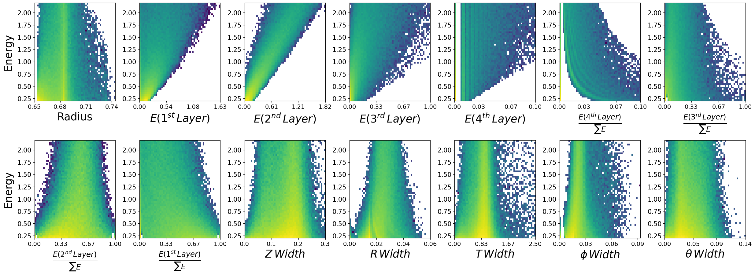
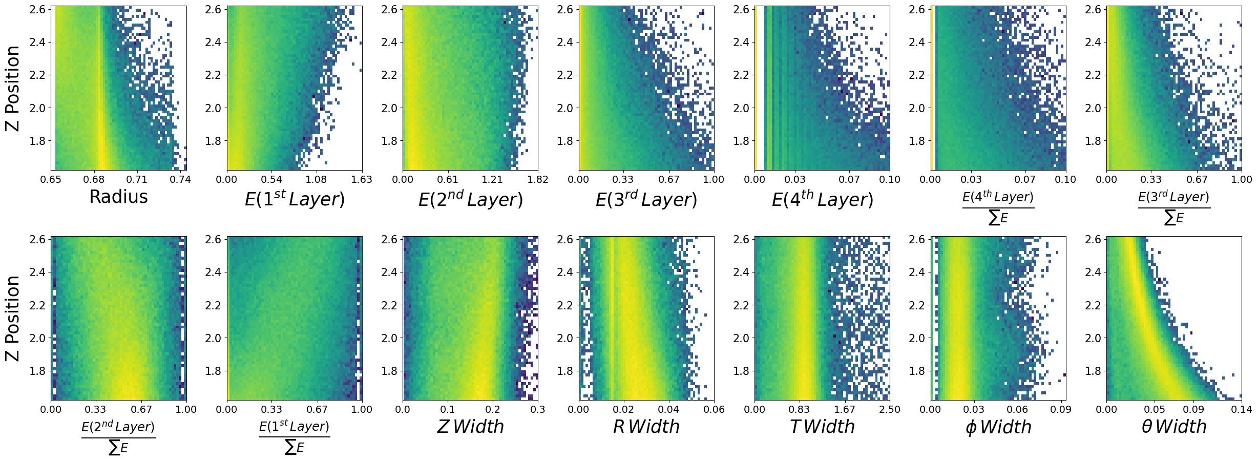
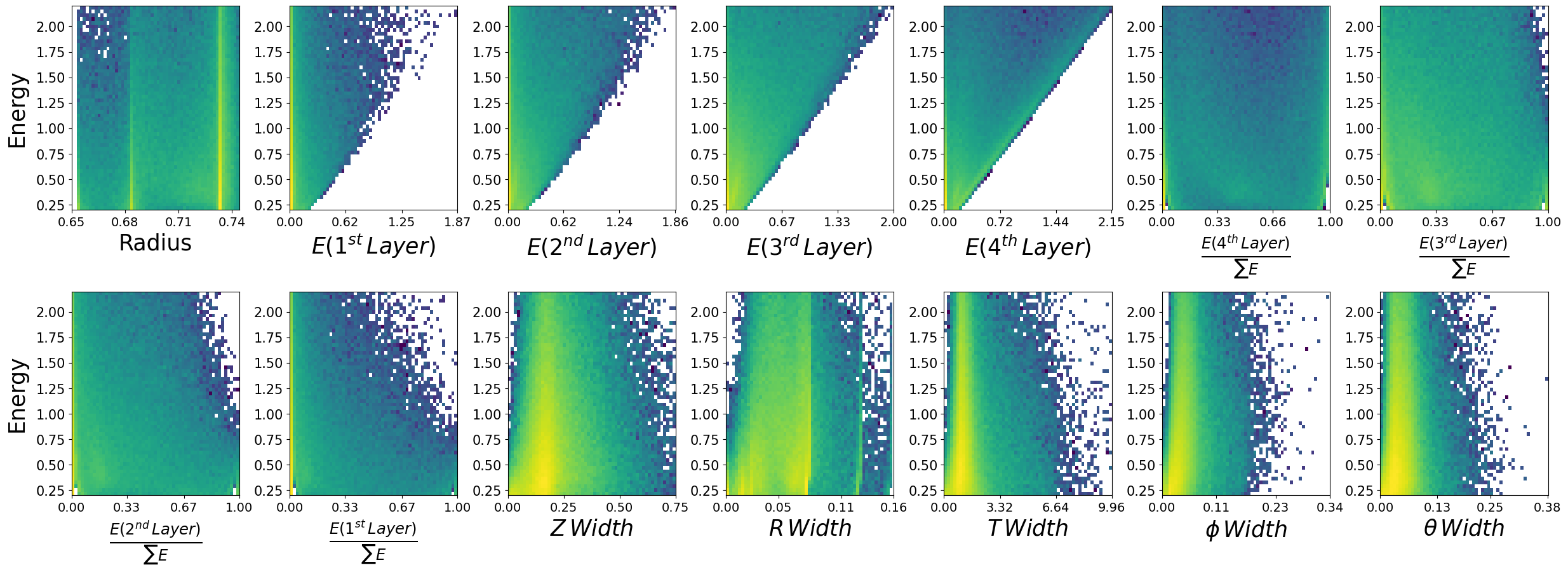
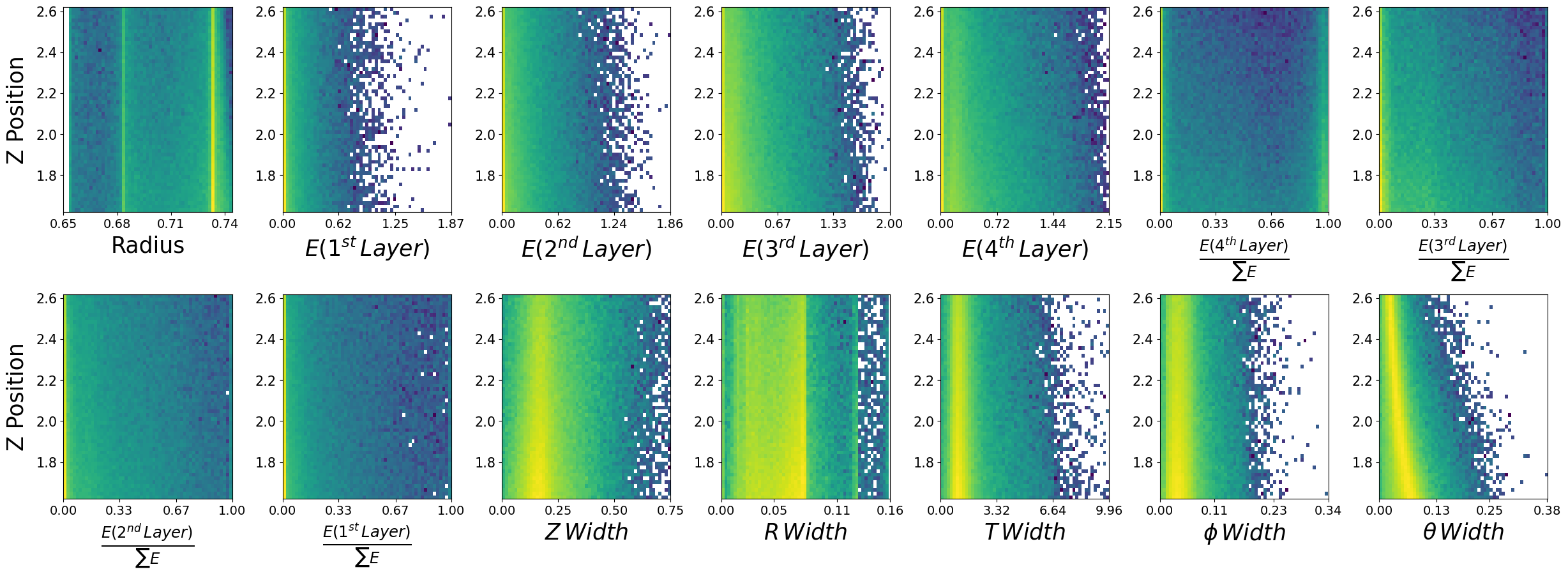
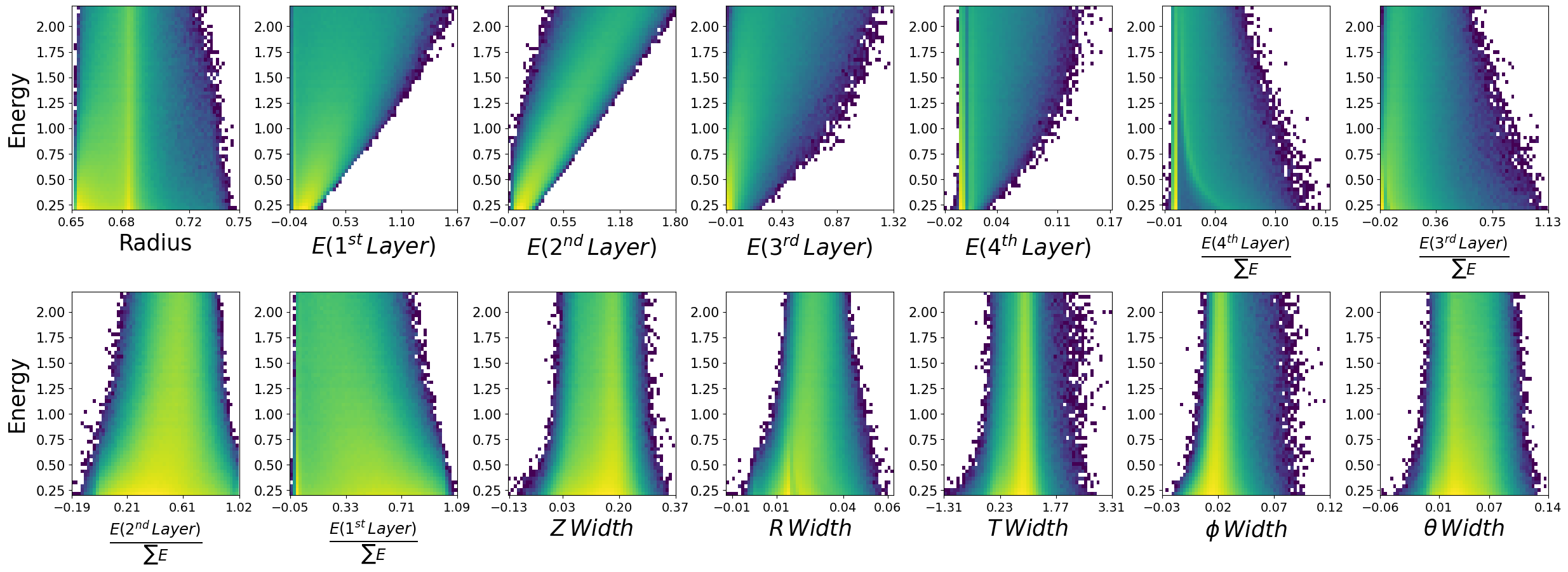
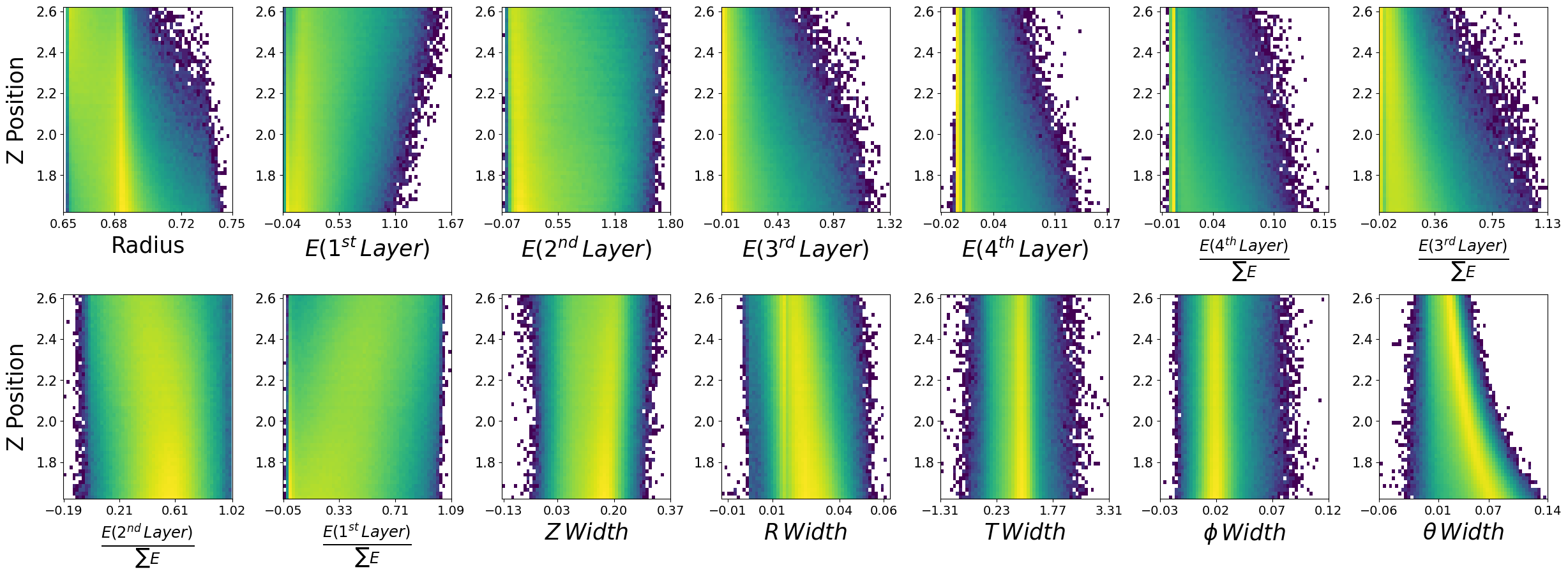
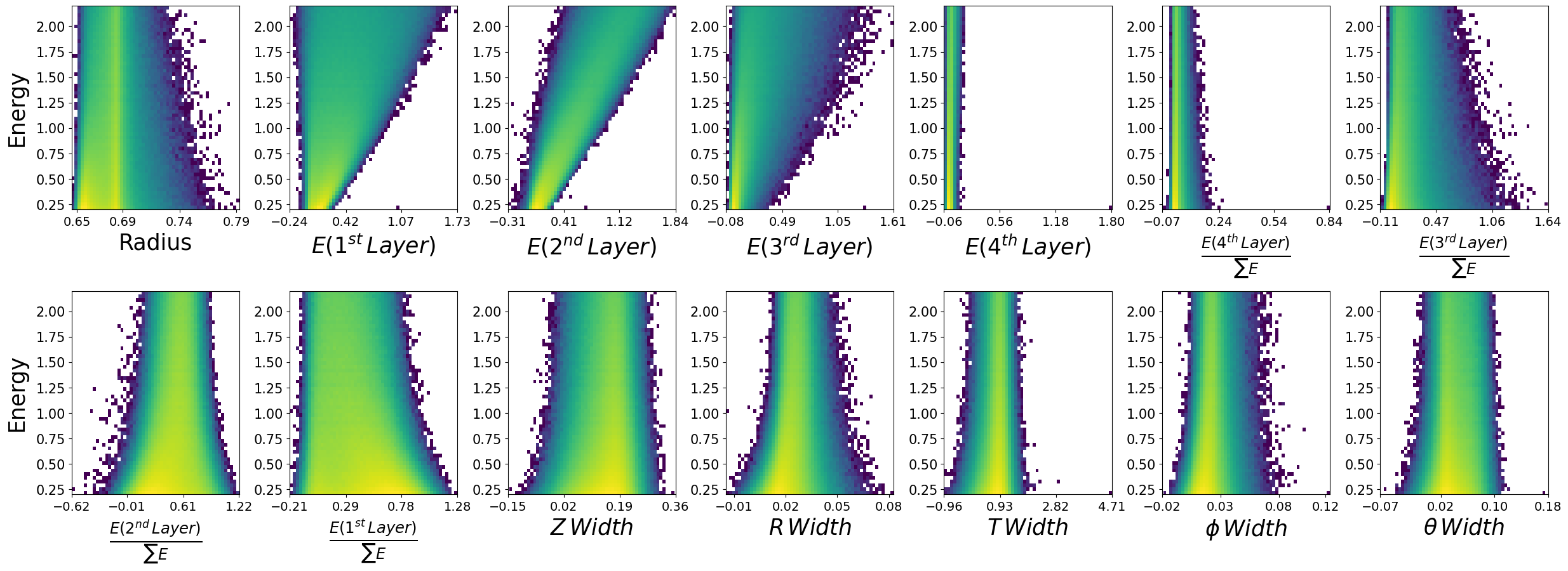
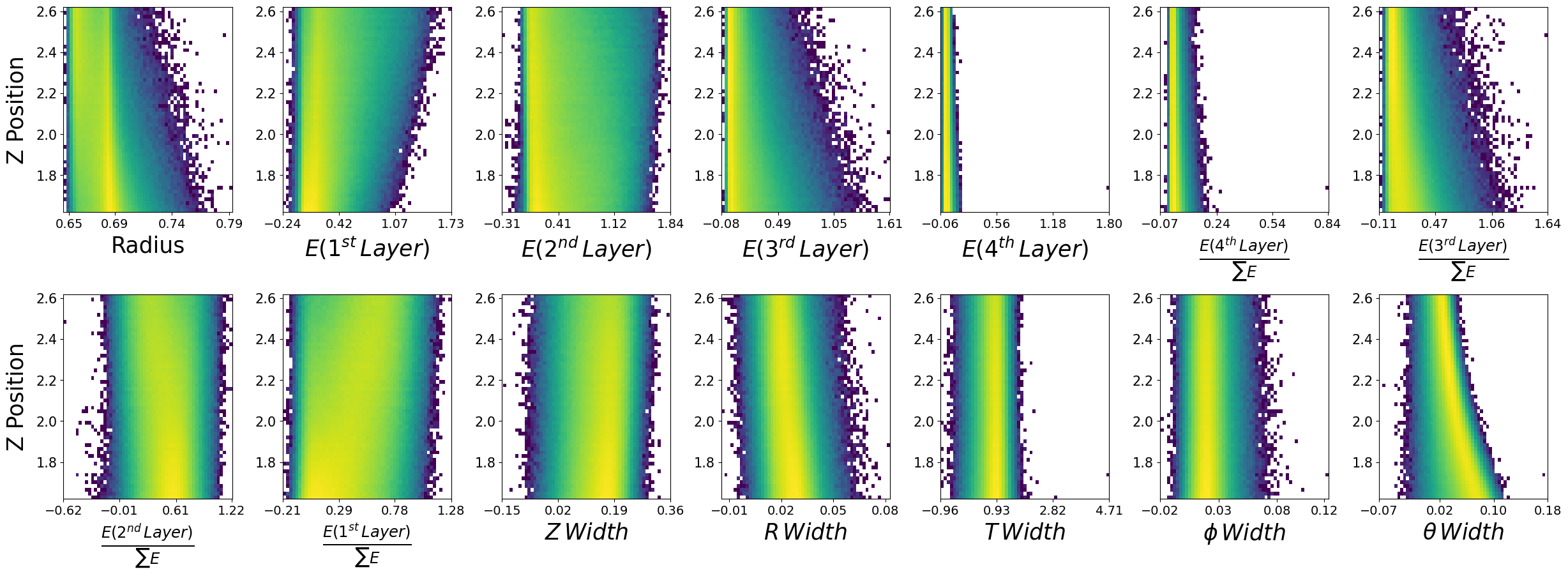
Lets look at how the features are distributed for both photons and neutrons, as a function of the two kinematic variables.
\(\boldsymbol{z}\) - recon_BCAL_z_entry
This is the z position (along the beamline) that a particle interacts with the innermost layer of the BCAL. The shower profile will change with a function of z. Does this make sense to you?
\(\boldsymbol{E}\) - recon_BCAL_E
The total reconstructed (by the detector) energy of a particle. The shower profile will change as a function of energy? Does this make sense to you?
import numpy as np
import matplotlib.pyplot as plt
import matplotlib as mpl

def make_plots(dataset,particle):
    columns = ['recon_BCAL_r', 'recon_BCAL_Layer1_E', 'recon_BCAL_Layer2_E',
           'recon_BCAL_Layer3_E', 'recon_BCAL_Layer4_E',
           'recon_BCAL_Layer4bySumLayers_E', 'recon_BCAL_Layer3bySumLayers_E',
           'recon_BCAL_Layer2bySumLayers_E', 'recon_BCAL_Layer1bySumLayers_E',
           'recon_BCAL_ZWidth', 'recon_BCAL_RWidth', 'recon_BCAL_TWidth',
           'recon_BCAL_PhiWidth', 'recon_BCAL_ThetaWidth']
    fig, axs = plt.subplots(2,7, figsize=(30, 10), facecolor='w', edgecolor='k')
    fig.subplots_adjust(hspace = 0.4, wspace=.3)
    axs = axs.ravel()


    labels = ['Radius',
     r'$E (1^{st} \, Layer)$',
     r'$E (2^{nd} \, Layer)$',
     r'$E (3^{rd} \, Layer)$',
     r'$E (4^{th} \, Layer)$',
     r'$\frac{E (4^{th} \, Layer)}{\sum E}$',
     r'$\frac{E (3^{rd} \, Layer)}{\sum E}$',
     r'$\frac{E (2^{nd} \, Layer)}{\sum E}$',
     r'$\frac{E (1^{st} \, Layer)}{\sum E}$',
     r'$Z \, Width$',
     r'$R \, Width$',
     r'$T \, Width$',
     r'$\phi \,  Width$',
     r'$\theta  \, Width$']

    i = 0
    print(particle)
    for column in columns:
        y = dataset[column]
        x = dataset['recon_BCAL_E']
        axs[i].hist2d(y,x,bins=55,density=True,alpha=1.0,norm=mpl.colors.LogNorm())
        plt.setp(axs[i].get_xticklabels(), fontsize=14)
        plt.setp(axs[i].get_yticklabels(), fontsize=15)
        ticks = np.linspace(min(y),max(y),4)
        ticks = np.around(ticks,decimals=2)
        axs[i].set_xticks(ticks=ticks)

        s = labels[i]

        axs[i].set_xlabel(s,fontsize=25,labelpad=5)
        if ((i == 0) or (i == 7)):
            axs[i].set_ylabel('Energy',fontsize=25,labelpad=9)
        i+=1

    N = len(columns)
    for ax in axs.flat[N:]:
        ax.remove()

    plt.show()
    plt.close()

    fig, axs = plt.subplots(2,7, figsize=(30, 10), facecolor='w', edgecolor='k')
    fig.subplots_adjust(hspace = 0.4, wspace=.3)
    axs = axs.ravel()

    i = 0
    for column in columns:
        y = dataset[column]
        x = dataset['recon_BCAL_z_entry']
        axs[i].hist2d(y,x,bins=55,density=True,alpha=1.0,norm=mpl.colors.LogNorm())
        plt.setp(axs[i].get_xticklabels(), fontsize=14)
        plt.setp(axs[i].get_yticklabels(), fontsize=15)  #to Set Matplotlib Tick Labels Font Size.
        ticks = np.linspace(min(y),max(y),4)
        ticks = np.around(ticks,decimals=2)
        axs[i].set_xticks(ticks=ticks)
        s = labels[i]

        axs[i].set_xlabel(s,fontsize=25,labelpad=5)
        if ((i == 0) or (i == 7)):
            axs[i].set_ylabel('Z Position',fontsize=25,labelpad=9)
        i+=1

    N = len(columns)
    for ax in axs.flat[N:]:
        ax.remove()

    plt.show()
    plt.close()
make_plots(photons,"Photons")
Photons
make_plots(neutrons,"Neutrons")
Neutrons
10.2. Data visualization is important#
We have expected distributions of the features as a function of the two kinematic parameters. This will be useful later for comparisons. We can generate artificial data with out network and check if the relationships are retained.
Now lets work on making methods to load the data into our models using standard pytorch functions.
I am going to introduce you to two different methods.
Custom Datasets
Dataloaders
Note that we don’t really need a custom dataset here and a simple TensorDataset() would do just fine, but lets use one anyways to get you more familiar with different pytorch methods.
Lets setup dictionaries of the normalization statistics of the two datasets, i.e., maximum and minimums. We could just use an sklearn method of MinMaxScaler() here, but lets consider a case when this is not feasible. For example, if we cannot fit all data into RAM and we need to load batches from file (not the case here, but you could face this).
One could precompute the statistics and load individual files to create the batches, scaling in the way we will define below.
fields = photons.columns

stats = {}
for field in fields:
    p_max = photons[field].max()
    n_max = neutrons[field].max()
    p_min = photons[field].min()
    n_min = neutrons[field].min()

    stats[f"{field}_max"] = max(p_max,n_max)
    stats[f"{field}_min"] = min(p_min,n_min)
stats
{'recon_BCAL_z_entry_max': np.float64(2.6199997),
 'recon_BCAL_z_entry_min': np.float64(1.6200029),
 'recon_BCAL_E_max': np.float64(2.1999831),
 'recon_BCAL_E_min': np.float64(0.2000011),
 'recon_BCAL_r_max': np.float64(0.74404915),
 'recon_BCAL_r_min': np.float64(0.65299995),
 'recon_BCAL_Layer1_E_max': np.float64(1.8684639),
 'recon_BCAL_Layer1_E_min': np.float64(0.0),
 'recon_BCAL_Layer2_E_max': np.float64(1.8641225),
 'recon_BCAL_Layer2_E_min': np.float64(0.0),
 'recon_BCAL_Layer3_E_max': np.float64(2.002063),
 'recon_BCAL_Layer3_E_min': np.float64(0.0),
 'recon_BCAL_Layer4_E_max': np.float64(2.1544363),
 'recon_BCAL_Layer4_E_min': np.float64(0.0),
 'recon_BCAL_Layer4bySumLayers_E_max': np.float64(0.99562687),
 'recon_BCAL_Layer4bySumLayers_E_min': np.float64(0.0),
 'recon_BCAL_Layer3bySumLayers_E_max': np.float64(1.0),
 'recon_BCAL_Layer3bySumLayers_E_min': np.float64(0.0),
 'recon_BCAL_Layer2bySumLayers_E_max': np.float64(1.0),
 'recon_BCAL_Layer2bySumLayers_E_min': np.float64(0.0),
 'recon_BCAL_Layer1bySumLayers_E_max': np.float64(1.0),
 'recon_BCAL_Layer1bySumLayers_E_min': np.float64(0.0),
 'recon_BCAL_ZWidth_max': np.float64(0.7497995999999999),
 'recon_BCAL_ZWidth_min': np.float64(0.00046754237),
 'recon_BCAL_RWidth_max': np.float64(0.158894415),
 'recon_BCAL_RWidth_min': np.float64(5.087822e-09),
 'recon_BCAL_TWidth_max': np.float64(9.955425),
 'recon_BCAL_TWidth_min': np.float64(6.242522e-05),
 'recon_BCAL_PhiWidth_max': np.float64(0.33884382),
 'recon_BCAL_PhiWidth_min': np.float64(1.1770585e-12),
 'recon_BCAL_ThetaWidth_max': np.float64(0.38148192),
 'recon_BCAL_ThetaWidth_min': np.float64(0.0002796732)}
import numpy as np
import pandas as pd
import random
from torch.utils.data import Dataset
import torch

class BCALDataset(Dataset):
    def __init__(self,dataset,mode="Single",stats=None):
        if mode is None:
            print("Please select one of the following modes:")
            print("1. Single")
            print("2. Combined")
            exit()
        self.stats = stats

        if self.stats is not None:
            self.max_values = np.array([self.stats[key] for key in list(self.stats.keys())[4:] if key.endswith('_max')])
            self.min_values = np.array([self.stats[key] for key in list(self.stats.keys())[4:] if key.endswith('_min')])
            self.max_conds = np.array([self.stats[key] for key in list(self.stats.keys())[:4] if key.endswith('_max')])
            self.min_conds = np.array([self.stats[key] for key in list(self.stats.keys())[:4] if key.endswith('_min')])

        else:
            print("Applying no scaling to your data.")

        if mode == "Single":
            self.data = dataset

        elif mode == "Combined":
            print('You need to write some code!')
            exit()
            # I leave this up to you.
            # Is it possible to combine the two particles under one model?
            # What else would you need to add?
            # Hint: Perhaps another conditional parameter corresponding to the PID (label)?
        else:
            print("Error in dataset creation. Exiting")
            exit()

    def __len__(self):
        return len(self.data)

    def scale_features(self,data):
        return 2.0 * (data - self.min_values) / (self.max_values - self.min_values) - 1.0 # (-1,1)

    def scale_conditions(self,conditions):
        return (conditions - self.min_conds) / (self.max_conds - self.min_conds) # (0,1)

    def __getitem__(self, idx):
        # Get the sample
        data = self.data[idx]
        conditions = data[:2]
        features = data[2:]
        unscaled_conditions = conditions.copy()

        if self.stats is not None:
            conditions = self.scale_conditions(conditions)
            features = self.scale_features(features)

       # PID = data[-1]   # Incase you want to get creative and combine the models. How could we use a PID?

        return features,conditions,unscaled_conditions
Lets take a look at how this works.
In pytorch when we create a custom dataset we will pass this to a “DataLoader”. The dataloader is simple a method of providing indicies to our getitem() function. All custom datasets need to have this function in order for the dataloader to be able to properly return batches!
With custom datasets we are able to have better control over our loading pipeline. As mentioned before, consider the case where you have large inputs that cannot all fit into RAM at once. Instead of grabbing a specific index of a preloaded numpy array (as above) we could load individual numpy files and create batches this way inside the getitem() function.
photon_dataset = BCALDataset(dataset=photons.to_numpy(),stats=stats,mode='Single')
Lets grab one item from our dataset and see what it looks like.
features,conditions,unscaled_conditions = photon_dataset.__getitem__(0)

print("Scaled Features")
print(features)
print("Scaled Conditions")
print(conditions)
print("Conditions")
print(unscaled_conditions)

del photon_dataset
Scaled Features
[-0.3991721  -0.40765139 -0.19837827 -0.71272782 -0.98625145 -0.98143995
 -0.64119646 -0.0677566  -0.3095258  -0.54592446 -0.61825955 -0.80214282
 -0.88954777 -0.75460464]
Scaled Conditions
[0.26407545 0.73630133]
Conditions
[1.8840775 1.6725905]
10.3. DataLoaders#
Now that we have an object that can sufficiently provide data to your network. We need to wrap it with a DataLoader() from pytorch. Why?
A pytorch dataloader takes as input some sort of Dataset object. It will then look at the entire length of the dataset and precompute a series of indices to form batches. For example, lets say our batch size is 5, the dataloader will produce something as follows:
\(B_1 = [0,10,25,45,21]\)
\(B_2 = [14,13,22,16,99]\)
Each of these integers is simply an index! This will produce a tensor of shape (5,features).
Now lets also make a custom collate function. A collate function simply tells the dataloader how I want you to format the output from my dataset.
from torch.utils.data import DataLoader

def BCAL_Collate(batch):
    features = []
    conditions = []
    unscaled = []
    # PIDs = []

    for f,c,uc in batch:
        features.append(torch.tensor(f))
        conditions.append(torch.tensor(c))
        unscaled.append(torch.tensor(uc))

    return torch.stack(features),torch.stack(conditions),torch.stack(unscaled)

# Create dataloaders to iterate.
def CreateLoaders(train_dataset,val_dataset,test_dataset,train_batch,val_batch,test_batch):
    train_loader = DataLoader(train_dataset,
                            batch_size=train_batch,
                            shuffle=True,collate_fn=BCAL_Collate,num_workers=0,pin_memory=False)
    val_loader =  DataLoader(val_dataset,
                            batch_size=val_batch,
                            shuffle=False,collate_fn=BCAL_Collate,num_workers=0,pin_memory=False)
    test_loader =  DataLoader(test_dataset,
                            batch_size=val_batch,
                            shuffle=False,collate_fn=BCAL_Collate,num_workers=0,pin_memory=False)
    return train_loader,val_loader,test_loader
Note that once again we do not need a custom collate function. Our data is a simple tabular format and pytorch has prebuilt functions (TensorDataset() and its collate function) that would handle this. But lets be complete.
Notice some of the arguments in the above DataLoader() functions. Here we control the batch size, whether we want to shuffle indices between epochs, etc. There are other arguments that are not extremely important here such as. You can see how these work in more complex environments here: https://pytorch.org/docs/stable/data.html
We have one more thing to do, we need to make a train,val,test split. We can use sklearn() functions to do this, or we can do it manually.
def create_train_test_split(dataset):
    Nt = int(0.7 * len(dataset))
    train = dataset[:Nt]
    test_val = dataset[Nt:]

    Nv = int(0.5 *len(test_val))
    val = test_val[:Nv]
    test = test_val[Nv:]
    print("Total dataset size: ",len(dataset))
    print("Number of Training data points: ",len(train))
    print("Number of Validation data points: ",len(val))
    print("Number of Testing data points: ",len(test))

    return train,val,test

training_photons,validation_photons,testing_photons = create_train_test_split(photons.to_numpy())
Total dataset size:  1726143
Number of Training data points:  1208300
Number of Validation data points:  258921
Number of Testing data points:  258922
Now lets complete the entire dataloading pipeline.
train_photons = BCALDataset(dataset=training_photons,mode="Single",stats=stats)
val_photons = BCALDataset(dataset=validation_photons,mode="Single",stats=stats)
test_photons = BCALDataset(dataset=testing_photons,mode="Single",stats=stats)

# Lets use batch sizes of 2048

train_batch_size = 2048
val_batch_size = 2048
test_batch_size = 2048

train_loader,val_loader,test_loader = CreateLoaders(train_photons,val_photons,test_photons,train_batch_size,val_batch_size,test_batch_size)
Now we can simple iterate the dataset as below. Being that you all have GPU access, we will make a simple assumption and put everything to GPU by default in training.
for i,data in enumerate(train_loader):
    print("Features: ",data[0])
    print("Scaled Conditions: ",data[1])
    print("Conditions: ",data[2])
    break
Features:  tensor([[-0.7354, -0.2106, -0.5411,  ..., -0.8287, -0.8140, -0.8600],
        [-0.6728, -0.7613, -0.7786,  ..., -0.8435, -0.8604, -0.7812],
        [-0.2396, -0.8950, -0.5691,  ..., -0.8763, -0.8800, -0.7680],
        ...,
        [-0.3499, -0.7163, -0.2374,  ..., -0.8462, -0.8497, -0.8275],
        [-0.3429, -0.9872, -0.8199,  ..., -0.9282, -0.9035, -0.8993],
        [-0.4345, -0.8280, -0.6824,  ..., -0.8335, -0.9009, -0.8599]],
       dtype=torch.float64)
Scaled Conditions:  tensor([[0.8422, 0.5379],
        [0.2350, 0.1472],
        [0.0269, 0.3064],
        ...,
        [0.7731, 0.4733],
        [0.2441, 0.0265],
        [0.9440, 0.1847]], dtype=torch.float64)
Conditions:  tensor([[2.4622, 1.2758],
        [1.8550, 0.4944],
        [1.6469, 0.8129],
        ...,
        [2.3931, 1.1465],
        [1.8641, 0.2531],
        [2.5640, 0.5693]], dtype=torch.float64)
10.4. The model#
This is fairly complicated, but we have written it to be inclusive of everything you will need.
The functions we will be using are:
log_prob() -> for training.
_sample() -> for generation.
import torch.nn as nn
from FrEIA.modules.base import InvertibleModule
import warnings
from typing import Callable
import math
import numpy as np
import torch
import torch.nn as nn
import torch.nn.functional as F
from scipy.stats import special_ortho_group
import FrEIA.framework as Ff
import FrEIA.modules as Fm
from nflows.distributions.normal import ConditionalDiagonalNormal
from nflows.utils import torchutils
from typing import Union, Iterable, Tuple


class FreiaNet(nn.Module):
    def __init__(self,input_shape,layers,context_shape,embedding=False,hidden_units=512,num_blocks=2,stats=None,device='cuda'):
        super(FreiaNet, self).__init__()
        self.input_shape = input_shape
        self.layers = layers
        self.context_shape = context_shape
        self.embedding = embedding
        self.hidden_units = hidden_units
        self.num_blocks = num_blocks
        self.device = device
        self.stats = stats

        if self.stats is not None:
            self.max_values = torch.tensor(np.array([self.stats[key] for key in list(self.stats.keys())[4:] if key.endswith('_max')])).to(device)
            self.min_values = torch.tensor(np.array([self.stats[key] for key in list(self.stats.keys())[4:] if key.endswith('_min')])).to(device)
            self.max_conds = torch.tensor(np.array([self.stats[key] for key in list(self.stats.keys())[:4] if key.endswith('_max')])).to(device)
            self.min_conds = torch.tensor(np.array([self.stats[key] for key in list(self.stats.keys())[:4] if key.endswith('_min')])).to(device)
        else:
            print("You have no included any stats for normalization values. Is this intentional?")

        if self.embedding:
            self.context_embedding = nn.Sequential(*[nn.Linear(context_shape,16),nn.ReLU(),nn.Linear(16,input_shape)])

        # Here we are setting up the conditional distribution
        # We will use an MLP to perform a learnable transformation on our conditions
        # The output of the MLP will characterize the mean and std of our Gaussian distribution
        context_encoder =  nn.Sequential(*[nn.Linear(context_shape,16),nn.ReLU(),nn.Linear(16,input_shape*2)])

        self.distribution = ConditionalDiagonalNormal(shape=[input_shape],context_encoder=context_encoder)

        # Create the bijective functions
        # Here we are combining FrEAI and NFlows
        # We will use the affine coupling transformation from FrEAI, but this entire function is derived from NFlows.
        def create_freai(input_shape,layer,cond_shape):
            inn = Ff.SequenceINN(input_shape)
            for k in range(layers):
                inn.append(Fm.AllInOneBlock,cond=0,cond_shape=(cond_shape,),subnet_constructor=subnet_fc, permute_soft=True)

            return inn

        def block(hidden_units):
            return [nn.Linear(hidden_units,hidden_units),nn.ReLU(),nn.Linear(hidden_units,hidden_units),nn.ReLU()]

        def subnet_fc(c_in, c_out):
            blks = [nn.Linear(c_in,hidden_units)]
            for _ in range(num_blocks):
                blks += block(hidden_units)

            blks += [nn.Linear(hidden_units,c_out)]
            return nn.Sequential(*blks)

        self.sequence = create_freai(self.input_shape,self.layers,self.context_shape)

    def log_prob(self,inputs,context):
        if self.embedding:
            embedded_context = self.context_embedding(context)
        else:
            embedded_context = context

        noise,logabsdet = self.sequence.forward(inputs,rev=False,c=[embedded_context])
        log_prob = self.distribution.log_prob(noise,context=embedded_context)

        return log_prob + logabsdet


    def __sample(self,num_samples,context):
        if self.embedding:
            embedded_context = self.context_embedding(context)
        else:
            embedded_context = context

        noise = self.distribution.sample(num_samples,context=embedded_context)

        if embedded_context is not None:
            noise = torchutils.merge_leading_dims(noise, num_dims=2)
            embedded_context = torchutils.repeat_rows(
                embedded_context, num_reps=num_samples
            )

        samples, _ = self.sequence.forward(noise,rev=True,c=[embedded_context])

        return samples

    def unscale(self,x):
        return 0.5 * (x + 1) * (self.max_values - self.min_values) + self.min_values

    def _sample(self,num_samples,context):
        samples = self.__sample(num_samples,context)
        samples = self.unscale(samples)
        return samples.detach().cpu().numpy()


    def sample_and_log_prob(self,num_samples,context):
        if self.embedding:
            embedded_context = self._embedding_net(context)
        else:
            embedded_context = context

        noise, log_prob = self.distribution.sample_and_log_prob(
            num_samples, context=embedded_context
        )

        if embedded_context is not None:
            # Merge the context dimension with sample dimension in order to apply the transform.
            noise = torchutils.merge_leading_dims(noise, num_dims=2)
            embedded_context = torchutils.repeat_rows(
                embedded_context, num_reps=num_samples
            )
        samples, logabsdet = self.sequence.forward(noise,rev=True,c=[embedded_context])

        if embedded_context is not None:
            # Split the context dimension from sample dimension.
            samples = torchutils.split_leading_dim(samples, shape=[-1, num_samples])
            logabsdet = torchutils.split_leading_dim(logabsdet, shape=[-1, num_samples])

        samples = self.unscale(samples)

        return samples.detach().cpu().numpy(), (log_prob - logabsdet).detach().cpu().numpy()


# Lets make a model. We will use the following parameters:
# input_shape,layers,context_shape,embedding=False,hidden_units=512,num_blocks=2
input_shape = 14 # the number of features we have
layers = 8 # how many chained bijections do we want to use i.e., f(f(f(x)))
context_shape = 2 # Number of conditional parameters
hidden_units = 256 # Recall that in our affine function we parameterize part of the transformation with a neural network.
                   # This controls how many "nodes" we want to use at each layer of this neural network
num_blocks = 2     # How many instances of the NN we use in the affine function -> see block() function above.
# stats = stats -> we will simply use the predefined statistics from above

photon_network = FreiaNet(input_shape=input_shape,layers=layers,context_shape=context_shape,hidden_units=hidden_units,num_blocks=num_blocks,stats=stats)
photon_network
FreiaNet(
  (distribution): ConditionalDiagonalNormal(
    (_context_encoder): Sequential(
      (0): Linear(in_features=2, out_features=16, bias=True)
      (1): ReLU()
      (2): Linear(in_features=16, out_features=28, bias=True)
    )
  )
  (sequence): SequenceINN(
    (module_list): ModuleList(
      (0-7): 8 x AllInOneBlock(
        (softplus): Softplus(beta=0.5, threshold=20.0)
        (subnet): Sequential(
          (0): Linear(in_features=9, out_features=256, bias=True)
          (1): Linear(in_features=256, out_features=256, bias=True)
          (2): ReLU()
          (3): Linear(in_features=256, out_features=256, bias=True)
          (4): ReLU()
          (5): Linear(in_features=256, out_features=256, bias=True)
          (6): ReLU()
          (7): Linear(in_features=256, out_features=256, bias=True)
          (8): ReLU()
          (9): Linear(in_features=256, out_features=14, bias=True)
        )
      )
    )
  )
)
10.5. Training function#
Lets write the training function in such a way that we can use it for any network, i.e., photons or neutrons.
There are two main components:
Training loop
Validation loop
We also need a clever way to store our parameters. Lets use a dictionary to do this.
config = {"seed":8,
          "name": "MyPhotonFlow",
          "run_val":1,
          "stats" :stats,
          "model": {
               "num_layers":8,
               "input_shape":14,
               "cond_shape":2,
               "num_blocks":2,
               "hidden_nodes": 512
           },
          "optimizer": {
                "lr": 7e-4,
            },
          "num_epochs": 50,
          "dataloader": {
            "train": {
                "batch_size": 2048
            },
            "val": {
                "batch_size": 2048
            },
            "test": {
                "batch_size": 25
            },
          },
            "output": {
                "dir":"./"
            }
}
import os
import json
import random
import pkbar
import torch.optim as optim
from torch.optim import lr_scheduler
import torch.nn as nn
import datetime
import shutil
import time

def trainer(config,dataset):
    # Setup random seed
    torch.manual_seed(config['seed'])
    np.random.seed(config['seed'])
    random.seed(config['seed'])
    torch.cuda.manual_seed(config['seed'])

    # Create experiment name
    exp_name = config['name']
    print(exp_name)

    # Create directory structure
    output_folder = config['output']['dir']
    output_path = os.path.join(output_folder,exp_name)
    os.makedirs(output_path,exist_ok=True)

    with open(os.path.join(output_path,'config.json'),'w') as outfile:
        json.dump(config, outfile)


       # Load the dataset
    print('Creating Loaders.')
    stats = config['stats']
    # Create datasets
    train,val,test = create_train_test_split(dataset.to_numpy())
    train = BCALDataset(dataset=train,mode="Single",stats=stats)
    val = BCALDataset(dataset=val,mode="Single",stats=stats)
    test_photons = BCALDataset(dataset=test,mode="Single",stats=stats)

    train_batch_size = config['dataloader']['train']['batch_size']
    val_batch_size = config['dataloader']['val']['batch_size']
    test_batch_size = config['dataloader']['val']['batch_size']

    train_loader,val_loader,test_loader = CreateLoaders(train,val,test,train_batch_size,val_batch_size,test_batch_size)

    history = {'train_loss':[],'val_loss':[],'lr':[]}


    print("Training Size: {0}".format(len(train_loader.dataset)))
    print("Validation Size: {0}".format(len(val_loader.dataset)))

    # Create the model
    num_layers = int(config['model']['num_layers'])
    input_shape = int(config['model']['input_shape'])
    cond_shape = int(config['model']['cond_shape'])
    num_blocks = int(config['model']['num_blocks'])
    hidden_nodes = int(config['model']['hidden_nodes'])
    net = FreiaNet(input_shape,num_layers,cond_shape,embedding=False,hidden_units=hidden_nodes,num_blocks=num_blocks,stats=stats)
    t_params = sum(p.numel() for p in net.parameters())
    print("Network Parameters: ",t_params)
    device = torch.device('cuda')
    net.to('cuda')

    # Optimizer
    num_epochs=int(config['num_epochs'])
    lr = float(config['optimizer']['lr'])

    optimizer = optim.Adam(list(filter(lambda p: p.requires_grad, net.parameters())), lr=lr)
    num_steps = len(train_loader) * num_epochs
    scheduler = torch.optim.lr_scheduler.CosineAnnealingLR(optimizer=optimizer, T_max=num_steps, last_epoch=-1,
                                                           eta_min=0)

    startEpoch = 0
    global_step = 0

    print('===========  Optimizer  ==================:')
    print('      LR:', lr)
    print('      num_epochs:', num_epochs)
    print('')

    for epoch in range(startEpoch,num_epochs):

        kbar = pkbar.Kbar(target=len(train_loader), epoch=epoch, num_epochs=num_epochs, width=20, always_stateful=False)

        net.train()
        running_loss = 0.0

        for i, data in enumerate(train_loader):
            input  = data[0].to('cuda').float()
            k = data[1].to('cuda').float()

            optimizer.zero_grad()

            with torch.set_grad_enabled(True):
                loss = -net.log_prob(inputs=input,context=k).mean()

            loss.backward()
            torch.nn.utils.clip_grad_norm_(net.parameters(), max_norm=0.5,error_if_nonfinite=True)
            optimizer.step()
            scheduler.step()

            running_loss += loss.item() * input.shape[0]
            kbar.update(i, values=[("loss", loss.item())])
            global_step += 1


        history['train_loss'].append(running_loss / len(train_loader.dataset))
        history['lr'].append(scheduler.get_last_lr()[0])


        ######################
        ## validation phase ##
        ######################
        if bool(config['run_val']):
            net.eval()
            val_loss = 0.0
            with torch.no_grad():
                for i, data in enumerate(val_loader):
                    input  = data[0].to('cuda').float()
                    k = data[1].to('cuda').float()
                    loss = -net.log_prob(inputs=input,context=k).mean()

                    val_loss += loss

            val_loss = val_loss.cpu().numpy() / len(val_loader)

            history['val_loss'].append(val_loss)

            kbar.add(1, values=[("val_loss", val_loss.item())])

            name_output_file = config['name']+'_epoch{:02d}_val_loss_{:.6f}.pth'.format(epoch, val_loss)

        else:
            kbar.add(1,values=[('val_loss',0.)])
            name_output_file = config['name']+'_epoch{:02d}_train_loss_{:.6f}.pth'.format(epoch, running_loss / len(train_loader.dataset))

        filename = os.path.join(output_path, name_output_file)

        checkpoint={}
        checkpoint['net_state_dict'] = net.state_dict()
        checkpoint['optimizer'] = optimizer.state_dict()
        checkpoint['scheduler'] = scheduler.state_dict()
        checkpoint['epoch'] = epoch
        checkpoint['history'] = history
        checkpoint['global_step'] = global_step

        torch.save(checkpoint,filename)

        print('')
trainer(config,photons)
MyPhotonFlow
Creating Loaders.
Total dataset size:  1726143
Number of Training data points:  1208300
Number of Validation data points:  258921
Number of Testing data points:  258922
Training Size: 1208300
Validation Size: 258921
Network Parameters:  8507292
===========  Optimizer  ==================:
      LR: 0.0007
      num_epochs: 50

Epoch: 1/50
590/590 [====================] - 32s 55ms/step - loss: -15.7588 - val_loss: -23.4704

Epoch: 2/50
590/590 [====================] - 33s 56ms/step - loss: -23.9841 - val_loss: -25.1621

Epoch: 3/50
590/590 [====================] - 35s 60ms/step - loss: -26.6910 - val_loss: -27.7281

Epoch: 4/50
590/590 [====================] - 33s 57ms/step - loss: -28.7214 - val_loss: -30.4870

Epoch: 5/50
590/590 [====================] - 32s 55ms/step - loss: -30.1571 - val_loss: -32.6433

Epoch: 6/50
590/590 [====================] - 33s 57ms/step - loss: -31.0260 - val_loss: -32.3942

Epoch: 7/50
590/590 [====================] - 33s 55ms/step - loss: -32.0959 - val_loss: -34.7934

Epoch: 8/50
590/590 [====================] - 33s 57ms/step - loss: -33.3529 - val_loss: -34.3647

Epoch: 9/50
590/590 [====================] - 33s 56ms/step - loss: -33.5115 - val_loss: -34.3981

Epoch: 10/50
590/590 [====================] - 33s 55ms/step - loss: -34.0910 - val_loss: -29.0998

Epoch: 11/50
590/590 [====================] - 33s 55ms/step - loss: -34.8968 - val_loss: -35.4194

Epoch: 12/50
590/590 [====================] - 32s 55ms/step - loss: -35.2383 - val_loss: -33.0309

Epoch: 13/50
590/590 [====================] - 33s 56ms/step - loss: -35.5779 - val_loss: -37.7742

Epoch: 14/50
590/590 [====================] - 34s 57ms/step - loss: -35.9140 - val_loss: -38.8968

Epoch: 15/50
590/590 [====================] - 34s 57ms/step - loss: -36.8263 - val_loss: -39.7397

Epoch: 16/50
590/590 [====================] - 33s 57ms/step - loss: -36.7026 - val_loss: -37.3383

Epoch: 17/50
590/590 [====================] - 33s 56ms/step - loss: -37.4666 - val_loss: -35.8774

Epoch: 18/50
590/590 [====================] - 33s 57ms/step - loss: -37.5883 - val_loss: -40.0610

Epoch: 19/50
590/590 [====================] - 34s 57ms/step - loss: -38.3701 - val_loss: -39.0972

Epoch: 20/50
590/590 [====================] - 32s 55ms/step - loss: -38.6748 - val_loss: -38.1420

Epoch: 21/50
590/590 [====================] - 36s 60ms/step - loss: -39.1797 - val_loss: -39.6254

Epoch: 22/50
590/590 [====================] - 35s 59ms/step - loss: -39.0675 - val_loss: -41.0746

Epoch: 23/50
590/590 [====================] - 35s 59ms/step - loss: -39.9491 - val_loss: -41.4044

Epoch: 24/50
590/590 [====================] - 35s 59ms/step - loss: -40.4717 - val_loss: -41.5697

Epoch: 25/50
590/590 [====================] - 33s 55ms/step - loss: -40.5598 - val_loss: -40.8873

Epoch: 26/50
590/590 [====================] - 32s 55ms/step - loss: -41.1005 - val_loss: -42.6984

Epoch: 27/50
590/590 [====================] - 33s 56ms/step - loss: -41.8666 - val_loss: -42.2635

Epoch: 28/50
590/590 [====================] - 32s 55ms/step - loss: -41.9345 - val_loss: -41.6732

Epoch: 29/50
590/590 [====================] - 33s 57ms/step - loss: -42.5932 - val_loss: -41.4016

Epoch: 30/50
590/590 [====================] - 33s 55ms/step - loss: -43.1504 - val_loss: -43.3892

Epoch: 31/50
590/590 [====================] - 32s 55ms/step - loss: -43.7098 - val_loss: -45.2355

Epoch: 32/50
590/590 [====================] - 33s 55ms/step - loss: -44.5343 - val_loss: -44.9671

Epoch: 33/50
590/590 [====================] - 33s 56ms/step - loss: -44.7599 - val_loss: -45.3687

Epoch: 34/50
590/590 [====================] - 32s 55ms/step - loss: -45.3550 - val_loss: -44.5358

Epoch: 35/50
590/590 [====================] - 33s 55ms/step - loss: -45.9191 - val_loss: -47.0917

Epoch: 36/50
590/590 [====================] - 32s 55ms/step - loss: -46.4677 - val_loss: -48.1689

Epoch: 37/50
590/590 [====================] - 32s 55ms/step - loss: -47.2344 - val_loss: -48.0064

Epoch: 38/50
590/590 [====================] - 33s 56ms/step - loss: -47.5051 - val_loss: -48.6606

Epoch: 39/50
590/590 [====================] - 33s 55ms/step - loss: -48.1256 - val_loss: -49.1900

Epoch: 40/50
590/590 [====================] - 33s 55ms/step - loss: -49.2798 - val_loss: -48.0611

Epoch: 41/50
590/590 [====================] - 32s 55ms/step - loss: -49.7005 - val_loss: -50.2045

Epoch: 42/50
590/590 [====================] - 32s 55ms/step - loss: -50.1377 - val_loss: -50.6557

Epoch: 43/50
590/590 [====================] - 33s 55ms/step - loss: -50.5644 - val_loss: -49.7120

Epoch: 44/50
590/590 [====================] - 33s 55ms/step - loss: -50.9958 - val_loss: -50.9747

Epoch: 45/50
590/590 [====================] - 32s 55ms/step - loss: -51.3898 - val_loss: -51.3880

Epoch: 46/50
590/590 [====================] - 32s 55ms/step - loss: -51.5960 - val_loss: -51.6131

Epoch: 47/50
590/590 [====================] - 32s 55ms/step - loss: -51.7696 - val_loss: -51.6693

Epoch: 48/50
590/590 [====================] - 33s 55ms/step - loss: -51.8873 - val_loss: -51.7486

Epoch: 49/50
590/590 [====================] - 32s 55ms/step - loss: -51.9543 - val_loss: -51.8091

Epoch: 50/50
590/590 [====================] - 32s 55ms/step - loss: -51.9883 - val_loss: -51.8207
10.6. Generations#
We have trained our model, and at each epoch we have saved the weights of the model to .pth file. This will be located in a folder corresponding to the “name” field of the config dictionary.
Lets load in the model, and create some generations. We will make the same plots as before and see if the relationships between E,z to each of the features is retained.
num_layers = int(config['model']['num_layers'])
input_shape = int(config['model']['input_shape'])
cond_shape = int(config['model']['cond_shape'])
num_blocks = int(config['model']['num_blocks'])
hidden_nodes = int(config['model']['hidden_nodes'])
net = FreiaNet(input_shape,num_layers,cond_shape,embedding=False,hidden_units=hidden_nodes,num_blocks=num_blocks,stats=stats)
t_params = sum(p.numel() for p in net.parameters())
print("Network Parameters: ",t_params)
device = torch.device('cuda')
net.to('cuda')

dicte = torch.load(os.path.join(config['name'],os.listdir(config['name'])[-1]))
net.load_state_dict(dicte["net_state_dict"])
Network Parameters: 8507292
/tmp/ipykernel_8616/1411825280.py:12: FutureWarning: You are using `torch.load` with `weights_only=False` (the current default value), which uses the default pickle module implicitly. It is possible to construct malicious pickle data which will execute arbitrary code during unpickling (See https://github.com/pytorch/pytorch/blob/main/SECURITY.md#untrusted-models for more details). In a future release, the default value for `weights_only` will be flipped to `True`. This limits the functions that could be executed during unpickling. Arbitrary objects will no longer be allowed to be loaded via this mode unless they are explicitly allowlisted by the user via `torch.serialization.add_safe_globals`. We recommend you start setting `weights_only=True` for any use case where you don't have full control of the loaded file. Please open an issue on GitHub for any issues related to this experimental feature.
  dicte = torch.load(os.path.join(config['name'],os.listdir(config['name'])[-1]))
<All keys matched successfully>
Lets create a dataloader that contains all the data. Realistically we only need the conditions!
all_data = BCALDataset(photons.to_numpy(),mode="Single",stats=stats)
all_loader = DataLoader(all_data,batch_size=10000)

net.eval() # Eval mode

generations = []
conditions = []
kbar = pkbar.Kbar(target=len(all_loader), width=20, always_stateful=False)
for i,data in enumerate(all_loader):
    kinematics = data[1].to('cuda').float()
    conditions.append(data[2].numpy())

    with torch.set_grad_enabled(False): # Same as with torch.no_grad():
        gens = net._sample(num_samples=1,context=kinematics)

    generations.append(gens)

    kbar.update(i)

generations = np.concatenate(generations)
conditions = np.concatenate(conditions)
172/173 [==================>.] - ETA: 0s
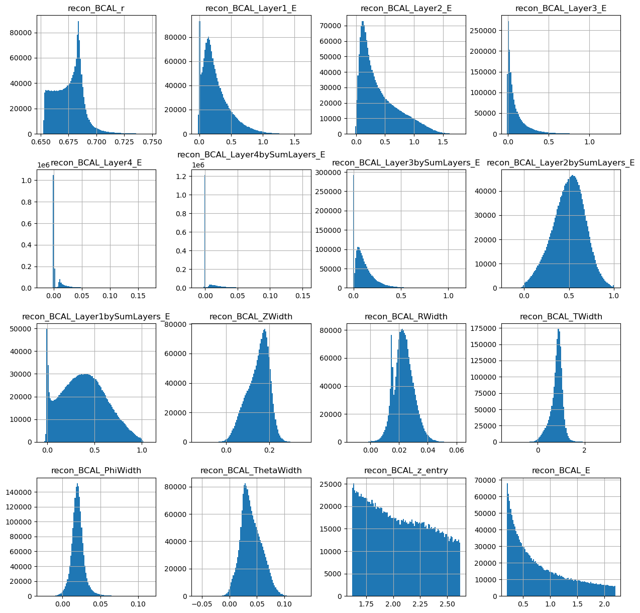
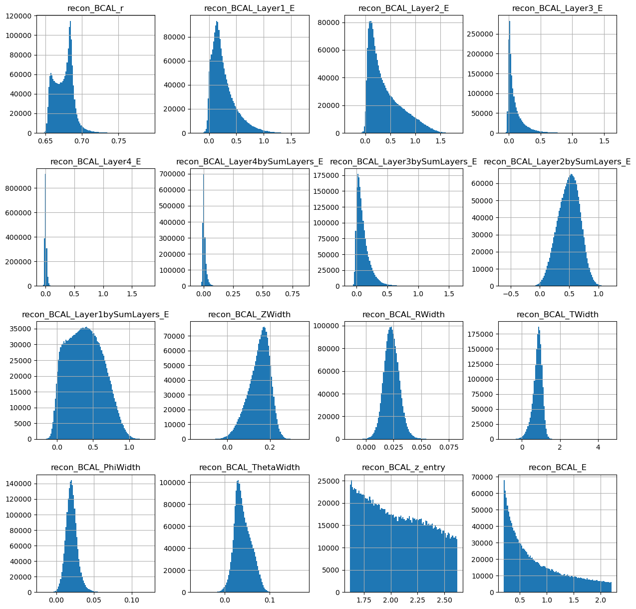
generated_dataframe = pd.DataFrame(generations,columns=photons.columns[2:])
generated_dataframe['recon_BCAL_z_entry'] = conditions[:,0]
generated_dataframe['recon_BCAL_E'] = conditions[:,1]

generated_dataframe.hist(bins=100,figsize=(15,15))
array([[<Axes: title={'center': 'recon_BCAL_r'}>,
        <Axes: title={'center': 'recon_BCAL_Layer1_E'}>,
        <Axes: title={'center': 'recon_BCAL_Layer2_E'}>,
        <Axes: title={'center': 'recon_BCAL_Layer3_E'}>],
       [<Axes: title={'center': 'recon_BCAL_Layer4_E'}>,
        <Axes: title={'center': 'recon_BCAL_Layer4bySumLayers_E'}>,
        <Axes: title={'center': 'recon_BCAL_Layer3bySumLayers_E'}>,
        <Axes: title={'center': 'recon_BCAL_Layer2bySumLayers_E'}>],
       [<Axes: title={'center': 'recon_BCAL_Layer1bySumLayers_E'}>,
        <Axes: title={'center': 'recon_BCAL_ZWidth'}>,
        <Axes: title={'center': 'recon_BCAL_RWidth'}>,
        <Axes: title={'center': 'recon_BCAL_TWidth'}>],
       [<Axes: title={'center': 'recon_BCAL_PhiWidth'}>,
        <Axes: title={'center': 'recon_BCAL_ThetaWidth'}>,
        <Axes: title={'center': 'recon_BCAL_z_entry'}>,
        <Axes: title={'center': 'recon_BCAL_E'}>]], dtype=object)
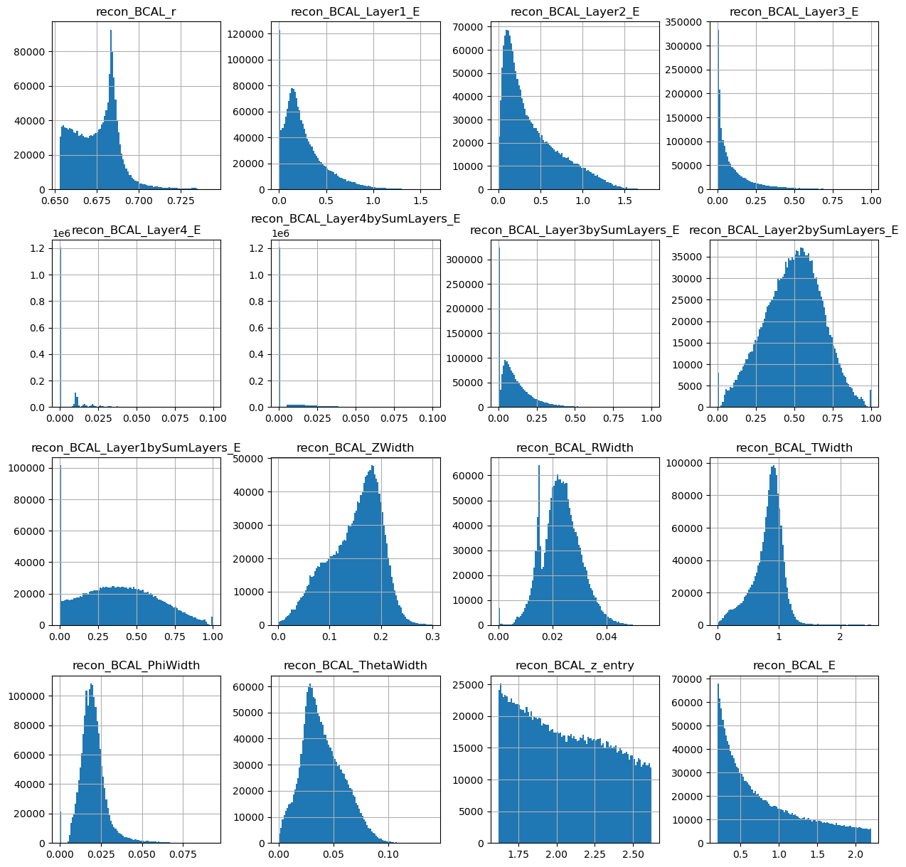
photons[generated_dataframe.columns].hist(figsize=(15,15),bins=100)
array([[<Axes: title={'center': 'recon_BCAL_r'}>,
        <Axes: title={'center': 'recon_BCAL_Layer1_E'}>,
        <Axes: title={'center': 'recon_BCAL_Layer2_E'}>,
        <Axes: title={'center': 'recon_BCAL_Layer3_E'}>],
       [<Axes: title={'center': 'recon_BCAL_Layer4_E'}>,
        <Axes: title={'center': 'recon_BCAL_Layer4bySumLayers_E'}>,
        <Axes: title={'center': 'recon_BCAL_Layer3bySumLayers_E'}>,
        <Axes: title={'center': 'recon_BCAL_Layer2bySumLayers_E'}>],
       [<Axes: title={'center': 'recon_BCAL_Layer1bySumLayers_E'}>,
        <Axes: title={'center': 'recon_BCAL_ZWidth'}>,
        <Axes: title={'center': 'recon_BCAL_RWidth'}>,
        <Axes: title={'center': 'recon_BCAL_TWidth'}>],
       [<Axes: title={'center': 'recon_BCAL_PhiWidth'}>,
        <Axes: title={'center': 'recon_BCAL_ThetaWidth'}>,
        <Axes: title={'center': 'recon_BCAL_z_entry'}>,
        <Axes: title={'center': 'recon_BCAL_E'}>]], dtype=object)
Looks ok. Lets make the same plots as we did from the true datasets.
make_plots(generated_dataframe,"Generated Photons")
Generated Photons
make_plots(photons,"True Photons")
True Photons
Not bad! Do you notice some things that are potentially wrong with the dataset we have generated? For example, what are the physical bounds of some of these features? This is something to think about with generative models in physics. In most cases, it is not enough to simply just generate data. One must come up with a scheme to ensure all samples generated are physical!
Can you think of ways to do this?
10.7. Flow Matching#
Now lets train a generative model using conditional Flow Matching. We will be able to use most of what we created above, we just need a seperate model class and a new training function.
from flow_matching.path.scheduler import CondOTScheduler
from flow_matching.path import AffineProbPath
from flow_matching.solver import Solver, ODESolver
from flow_matching.utils import ModelWrapper
from torch import Tensor
The base neural network structure - you are free to modify this later.
def antiderivTanh(x): # activation function aka the antiderivative of tanh
    return torch.abs(x) + torch.log(1+torch.exp(-2.0*torch.abs(x)))

def derivTanh(x): # act'' aka the second derivative of the activation function antiderivTanh
    return 1 - torch.pow( torch.tanh(x) , 2 )

class ResNN(nn.Module):
    def __init__(self, d, m, nTh=2,conditional_dim=2):
        super().__init__()

        if nTh < 2:
            print("nTh must be an integer >= 2")
            exit(1)

        self.d = d
        self.m = m
        self.nTh = nTh
        self.layers = nn.ModuleList([])
        self.layers.append(nn.Linear(d + 1 + conditional_dim, m, bias=True)) # opening layer
        self.layers.append(nn.Linear(m,m, bias=True)) # resnet layers
        for i in range(nTh-2):
            self.layers.append(copy.deepcopy(self.layers[1]))
        self.act = antiderivTanh
        self.h = 1.0 / (self.nTh-1) # step size for the ResNet
        self.output_layer = nn.Linear(m,d)

    def forward(self, x,t, c=None):
        t = t.reshape(-1,1).float()

        if c is None:
            x = self.act(self.layers[0].forward(torch.concat([x,t],-1)))
        else:
            x = self.act(self.layers[0].forward(torch.concat([x,c,t],dim=-1)))

        for i in range(1,self.nTh):
            x = x + self.h * self.act(self.layers[i](x))

        return self.output_layer(x)

    def step(self, x,t,c=None):
        t = t.reshape(-1, 1).expand(x.shape[0], 1)

        if c is None:
            x = self.act(self.layers[0].forward(torch.concat([x,t],-1)))
        else:
            x = self.act(self.layers[0].forward(torch.concat([x,c,t],dim=-1)))

        for i in range(1,self.nTh):
            x = x + self.h * self.act(self.layers[i](x))

        return self.output_layer(x)


# We need this to perform our numerical integration for generation.

class WrappedModel(ModelWrapper):
    def forward(self, x: torch.Tensor, t: torch.Tensor, **extras):
        c = extras.get("model_extras", {}).get("c", None)
        return self.model.step(x, t, c=c)
import copy

class FlowMatching(nn.Module):
    def __init__(self,input_shape,layers,context_shape,embedding=False,hidden_units=512,num_blocks=2,stats=None,device='cuda'):
        super(FlowMatching, self).__init__()
        self.input_shape = input_shape
        self.layers = layers
        self.context_shape = context_shape
        self.embedding = embedding
        self.hidden_units = hidden_units
        self.num_blocks = num_blocks
        self.device = device
        self.stats = stats

        if self.stats is not None:
            self.max_values = torch.tensor(np.array([self.stats[key] for key in list(self.stats.keys())[4:] if key.endswith('_max')])).to(device)
            self.min_values = torch.tensor(np.array([self.stats[key] for key in list(self.stats.keys())[4:] if key.endswith('_min')])).to(device)
            self.max_conds = torch.tensor(np.array([self.stats[key] for key in list(self.stats.keys())[:4] if key.endswith('_max')])).to(device)
            self.min_conds = torch.tensor(np.array([self.stats[key] for key in list(self.stats.keys())[:4] if key.endswith('_min')])).to(device)
        else:
            print("You have no included any stats for normalization values. Is this intentional?")

        if self.embedding:
            self.context_embedding = nn.Sequential(*[nn.Linear(context_shape,16),nn.ReLU(),nn.Linear(16,input_shape)])

        # Our neural network predicting the velocity field
        self.NN = ResNN(nTh=self.layers,m=self.hidden_units,d=self.input_shape,conditional_dim=self.context_shape)
        # Our path will follow exactly what we discussed in the slides
        self.path = AffineProbPath(scheduler=CondOTScheduler())


    # our loss function used for training - simple MSE between v_t and u_t
    def compute_loss(self, x_1, context):
        if self.embedding:
            embedded_context = self.context_embedding(context)
        else:
            embedded_context = context

        x_0 = torch.randn_like(x_1).to(x_1.device)

        t = torch.rand(x_1.shape[0]).to(x_1.device)

        path_sample = self.path.sample(t=t, x_0=x_0, x_1=x_1)

        loss = torch.pow( self.NN(x=path_sample.x_t,t=path_sample.t,c=embedded_context) - path_sample.dx_t, 2).mean()

        return loss

    # number of integration steps.
    def __sample(self,nt=20, context=None):
        if self.embedding:
            embedded_context = self.context_embedding(context)
        else:
            embedded_context = context

        wrapped_vf = WrappedModel(self.NN)
        step_size = 1.0 / (2*nt)
        T = torch.linspace(0,1,nt).to(self.device)

        x_init = torch.randn((context.shape[0], self.input_shape), dtype=torch.float32, device=self.device)
        # Solve the ODE
        solver = ODESolver(velocity_model=wrapped_vf)
        sol = solver.sample(time_grid=T, x_init=x_init, method='midpoint', step_size=step_size, return_intermediates=False,model_extras={"c": embedded_context})
        return sol

    def unscale(self,x):
        return 0.5 * (x + 1) * (self.max_values - self.min_values) + self.min_values

    def _sample(self,nt,context):
        samples = self.__sample(nt=nt,context=context)
        samples = self.unscale(samples)
        return samples.detach().cpu().numpy()
def trainer_fm(config,dataset):
    # Setup random seed
    torch.manual_seed(config['seed'])
    np.random.seed(config['seed'])
    random.seed(config['seed'])
    torch.cuda.manual_seed(config['seed'])

    # Create experiment name
    exp_name = config['name']
    print(exp_name)

    # Create directory structure
    output_folder = config['output']['dir']
    output_path = os.path.join(output_folder,exp_name)
    os.makedirs(output_path,exist_ok=True)

    with open(os.path.join(output_path,'config.json'),'w') as outfile:
        json.dump(config, outfile)


       # Load the dataset
    print('Creating Loaders.')
    stats = config['stats']
    # Create datasets
    train,val,test = create_train_test_split(dataset.to_numpy())
    train = BCALDataset(dataset=train,mode="Single",stats=stats)
    val = BCALDataset(dataset=val,mode="Single",stats=stats)
    test_photons = BCALDataset(dataset=test,mode="Single",stats=stats)

    train_batch_size = config['dataloader']['train']['batch_size']
    val_batch_size = config['dataloader']['val']['batch_size']
    test_batch_size = config['dataloader']['val']['batch_size']

    train_loader,val_loader,test_loader = CreateLoaders(train,val,test,train_batch_size,val_batch_size,test_batch_size)

    history = {'train_loss':[],'val_loss':[],'lr':[]}


    print("Training Size: {0}".format(len(train_loader.dataset)))
    print("Validation Size: {0}".format(len(val_loader.dataset)))

    # Create the model
    num_layers = int(config['model']['num_layers'])
    input_shape = int(config['model']['input_shape'])
    cond_shape = int(config['model']['cond_shape'])
    num_blocks = int(config['model']['num_blocks'])
    hidden_nodes = int(config['model']['hidden_nodes'])
    net = FlowMatching(input_shape,num_layers,cond_shape,embedding=False,hidden_units=hidden_nodes,num_blocks=num_blocks,stats=stats)
    t_params = sum(p.numel() for p in net.parameters())
    print("Network Parameters: ",t_params)
    device = torch.device('cuda')
    net.to('cuda')

    # Optimizer
    num_epochs=int(config['num_epochs'])
    lr = float(config['optimizer']['lr'])

    optimizer = optim.Adam(list(filter(lambda p: p.requires_grad, net.parameters())), lr=lr)
    num_steps = len(train_loader) * num_epochs
    scheduler = torch.optim.lr_scheduler.CosineAnnealingLR(optimizer=optimizer, T_max=num_steps, last_epoch=-1,
                                                           eta_min=0)

    startEpoch = 0
    global_step = 0

    print('===========  Optimizer  ==================:')
    print('      LR:', lr)
    print('      num_epochs:', num_epochs)
    print('')

    for epoch in range(startEpoch,num_epochs):

        kbar = pkbar.Kbar(target=len(train_loader), epoch=epoch, num_epochs=num_epochs, width=20, always_stateful=False)

        net.train()
        running_loss = 0.0

        for i, data in enumerate(train_loader):
            input  = data[0].to('cuda').float()
            k = data[1].to('cuda').float()

            optimizer.zero_grad()

            with torch.set_grad_enabled(True):
                loss = net.compute_loss(x_1=input,context=k)

            loss.backward()
            torch.nn.utils.clip_grad_norm_(net.parameters(), max_norm=0.5,error_if_nonfinite=True)
            optimizer.step()
            scheduler.step()

            running_loss += loss.item() * input.shape[0]
            kbar.update(i, values=[("loss", loss.item())])
            global_step += 1


        history['train_loss'].append(running_loss / len(train_loader.dataset))
        history['lr'].append(scheduler.get_last_lr()[0])


        ######################
        ## validation phase ##
        ######################
        if bool(config['run_val']):
            net.eval()
            val_loss = 0.0
            with torch.no_grad():
                for i, data in enumerate(val_loader):
                    input  = data[0].to('cuda').float()
                    k = data[1].to('cuda').float()
                    loss = net.compute_loss(x_1=input,context=k)

                    val_loss += loss

            val_loss = val_loss.cpu().numpy() / len(val_loader)

            history['val_loss'].append(val_loss)

            kbar.add(1, values=[("val_loss", val_loss.item())])

            name_output_file = config['name']+'_epoch{:02d}_val_loss_{:.6f}.pth'.format(epoch, val_loss)

        else:
            kbar.add(1,values=[('val_loss',0.)])
            name_output_file = config['name']+'_epoch{:02d}_train_loss_{:.6f}.pth'.format(epoch, running_loss / len(train_loader.dataset))

        filename = os.path.join(output_path, name_output_file)

        checkpoint={}
        checkpoint['net_state_dict'] = net.state_dict()
        checkpoint['optimizer'] = optimizer.state_dict()
        checkpoint['scheduler'] = scheduler.state_dict()
        checkpoint['epoch'] = epoch
        checkpoint['history'] = history
        checkpoint['global_step'] = global_step

        torch.save(checkpoint,filename)

        print('')
config_fm = {"seed":8,
          "name": "MyPhotonFlowMatching",
          "run_val":1,
          "stats" :stats,
          "model": {
               "num_layers":8,
               "input_shape":14,
               "cond_shape":2,
               "num_blocks":2,
               "hidden_nodes": 512
           },
          "optimizer": {
                "lr": 7e-4,
            },
          "num_epochs": 50,
          "dataloader": {
            "train": {
                "batch_size": 2048
            },
            "val": {
                "batch_size": 2048
            },
            "test": {
                "batch_size": 25
            },
          },
            "output": {
                "dir":"./"
            }
}
trainer_fm(config_fm,photons)
MyPhotonFlowMatching
Creating Loaders.
Total dataset size:  1726143
Number of Training data points:  1208300
Number of Validation data points:  258921
Number of Testing data points:  258922
Training Size: 1208300
Validation Size: 258921
Network Parameters:  1854990
===========  Optimizer  ==================:
      LR: 0.0007
      num_epochs: 50

Epoch: 1/50
590/590 [====================] - 26s 44ms/step - loss: 0.4484 - val_loss: 0.3051

Epoch: 2/50
590/590 [====================] - 26s 44ms/step - loss: 0.2520 - val_loss: 0.2257

Epoch: 3/50
590/590 [====================] - 26s 44ms/step - loss: 0.2081 - val_loss: 0.1924

Epoch: 4/50
590/590 [====================] - 26s 44ms/step - loss: 0.1879 - val_loss: 0.1844

Epoch: 5/50
590/590 [====================] - 26s 44ms/step - loss: 0.1780 - val_loss: 0.1797

Epoch: 6/50
590/590 [====================] - 26s 44ms/step - loss: 0.1711 - val_loss: 0.1695

Epoch: 7/50
590/590 [====================] - 26s 44ms/step - loss: 0.1689 - val_loss: 0.1629

Epoch: 8/50
590/590 [====================] - 26s 44ms/step - loss: 0.1647 - val_loss: 0.1572

Epoch: 9/50
590/590 [====================] - 26s 44ms/step - loss: 0.1624 - val_loss: 0.1551

Epoch: 10/50
590/590 [====================] - 26s 44ms/step - loss: 0.1605 - val_loss: 0.1595

Epoch: 11/50
590/590 [====================] - 26s 44ms/step - loss: 0.1595 - val_loss: 0.1690

Epoch: 12/50
590/590 [====================] - 26s 44ms/step - loss: 0.1579 - val_loss: 0.1583

Epoch: 13/50
590/590 [====================] - 26s 44ms/step - loss: 0.1563 - val_loss: 0.1607

Epoch: 14/50
590/590 [====================] - 26s 44ms/step - loss: 0.1553 - val_loss: 0.1552

Epoch: 15/50
590/590 [====================] - 26s 44ms/step - loss: 0.1541 - val_loss: 0.1517

Epoch: 16/50
590/590 [====================] - 26s 44ms/step - loss: 0.1540 - val_loss: 0.1505

Epoch: 17/50
590/590 [====================] - 26s 44ms/step - loss: 0.1525 - val_loss: 0.1548

Epoch: 18/50
590/590 [====================] - 26s 44ms/step - loss: 0.1518 - val_loss: 0.1476

Epoch: 19/50
590/590 [====================] - 26s 44ms/step - loss: 0.1501 - val_loss: 0.1511

Epoch: 20/50
590/590 [====================] - 26s 44ms/step - loss: 0.1493 - val_loss: 0.1475

Epoch: 21/50
590/590 [====================] - 26s 45ms/step - loss: 0.1490 - val_loss: 0.1484

Epoch: 22/50
590/590 [====================] - 26s 44ms/step - loss: 0.1482 - val_loss: 0.1495

Epoch: 23/50
590/590 [====================] - 26s 44ms/step - loss: 0.1479 - val_loss: 0.1459

Epoch: 24/50
590/590 [====================] - 26s 44ms/step - loss: 0.1468 - val_loss: 0.1457

Epoch: 25/50
590/590 [====================] - 26s 44ms/step - loss: 0.1460 - val_loss: 0.1461

Epoch: 26/50
590/590 [====================] - 26s 44ms/step - loss: 0.1454 - val_loss: 0.1452

Epoch: 27/50
590/590 [====================] - 26s 44ms/step - loss: 0.1449 - val_loss: 0.1449

Epoch: 28/50
590/590 [====================] - 26s 44ms/step - loss: 0.1442 - val_loss: 0.1451

Epoch: 29/50
590/590 [====================] - 26s 44ms/step - loss: 0.1442 - val_loss: 0.1446

Epoch: 30/50
590/590 [====================] - 26s 44ms/step - loss: 0.1430 - val_loss: 0.1435

Epoch: 31/50
590/590 [====================] - 26s 44ms/step - loss: 0.1428 - val_loss: 0.1429

Epoch: 32/50
590/590 [====================] - 26s 44ms/step - loss: 0.1424 - val_loss: 0.1426

Epoch: 33/50
590/590 [====================] - 26s 44ms/step - loss: 0.1414 - val_loss: 0.1406

Epoch: 34/50
590/590 [====================] - 26s 44ms/step - loss: 0.1414 - val_loss: 0.1417

Epoch: 35/50
590/590 [====================] - 26s 44ms/step - loss: 0.1408 - val_loss: 0.1407

Epoch: 36/50
590/590 [====================] - 26s 44ms/step - loss: 0.1407 - val_loss: 0.1399

Epoch: 37/50
590/590 [====================] - 26s 44ms/step - loss: 0.1402 - val_loss: 0.1406

Epoch: 38/50
590/590 [====================] - 26s 44ms/step - loss: 0.1398 - val_loss: 0.1398

Epoch: 39/50
590/590 [====================] - 26s 44ms/step - loss: 0.1395 - val_loss: 0.1392

Epoch: 40/50
590/590 [====================] - 26s 44ms/step - loss: 0.1392 - val_loss: 0.1392

Epoch: 41/50
590/590 [====================] - 26s 44ms/step - loss: 0.1391 - val_loss: 0.1385

Epoch: 42/50
590/590 [====================] - 26s 44ms/step - loss: 0.1388 - val_loss: 0.1391

Epoch: 43/50
590/590 [====================] - 26s 44ms/step - loss: 0.1388 - val_loss: 0.1388

Epoch: 44/50
590/590 [====================] - 26s 44ms/step - loss: 0.1382 - val_loss: 0.1385

Epoch: 45/50
590/590 [====================] - 26s 44ms/step - loss: 0.1382 - val_loss: 0.1383

Epoch: 46/50
590/590 [====================] - 26s 44ms/step - loss: 0.1384 - val_loss: 0.1377

Epoch: 47/50
590/590 [====================] - 26s 44ms/step - loss: 0.1381 - val_loss: 0.1382

Epoch: 48/50
590/590 [====================] - 29s 49ms/step - loss: 0.1379 - val_loss: 0.1386

Epoch: 49/50
590/590 [====================] - 26s 45ms/step - loss: 0.1378 - val_loss: 0.1380

Epoch: 50/50
590/590 [====================] - 26s 44ms/step - loss: 0.1380 - val_loss: 0.1385
num_layers = int(config_fm['model']['num_layers'])
input_shape = int(config_fm['model']['input_shape'])
cond_shape = int(config_fm['model']['cond_shape'])
num_blocks = int(config_fm['model']['num_blocks'])
hidden_nodes = int(config_fm['model']['hidden_nodes'])
net = FlowMatching(input_shape,num_layers,cond_shape,embedding=False,hidden_units=hidden_nodes,num_blocks=num_blocks,stats=stats)
t_params = sum(p.numel() for p in net.parameters())
print("Network Parameters: ",t_params)
device = torch.device('cuda')
net.to('cuda')

dicte = torch.load(os.path.join(config_fm['name'],os.listdir(config_fm['name'])[-1]))
net.load_state_dict(dicte["net_state_dict"])
Network Parameters: 1854990
/tmp/ipykernel_8616/203205216.py:12: FutureWarning: You are using `torch.load` with `weights_only=False` (the current default value), which uses the default pickle module implicitly. It is possible to construct malicious pickle data which will execute arbitrary code during unpickling (See https://github.com/pytorch/pytorch/blob/main/SECURITY.md#untrusted-models for more details). In a future release, the default value for `weights_only` will be flipped to `True`. This limits the functions that could be executed during unpickling. Arbitrary objects will no longer be allowed to be loaded via this mode unless they are explicitly allowlisted by the user via `torch.serialization.add_safe_globals`. We recommend you start setting `weights_only=True` for any use case where you don't have full control of the loaded file. Please open an issue on GitHub for any issues related to this experimental feature.
  dicte = torch.load(os.path.join(config_fm['name'],os.listdir(config_fm['name'])[-1]))
<All keys matched successfully>
all_data = BCALDataset(photons.to_numpy(),mode="Single",stats=stats)
all_loader = DataLoader(all_data,batch_size=10000)

net.eval() # Eval mode

generations = []
conditions = []
kbar = pkbar.Kbar(target=len(all_loader), width=20, always_stateful=False)
for i,data in enumerate(all_loader):
    kinematics = data[1].to('cuda').float()
    conditions.append(data[2].numpy())

    with torch.set_grad_enabled(False): # Same as with torch.no_grad():
        gens = net._sample(nt=20,context=kinematics) # You can play around with integration steps - if you want to experiment with different integration methods we can

    generations.append(gens)

    kbar.update(i)

generations = np.concatenate(generations)
conditions = np.concatenate(conditions)
172/173 [==================>.] - ETA: 0s
generated_dataframe = pd.DataFrame(generations,columns=photons.columns[2:])
generated_dataframe['recon_BCAL_z_entry'] = conditions[:,0]
generated_dataframe['recon_BCAL_E'] = conditions[:,1]

generated_dataframe.hist(bins=100,figsize=(15,15))
array([[<Axes: title={'center': 'recon_BCAL_r'}>,
        <Axes: title={'center': 'recon_BCAL_Layer1_E'}>,
        <Axes: title={'center': 'recon_BCAL_Layer2_E'}>,
        <Axes: title={'center': 'recon_BCAL_Layer3_E'}>],
       [<Axes: title={'center': 'recon_BCAL_Layer4_E'}>,
        <Axes: title={'center': 'recon_BCAL_Layer4bySumLayers_E'}>,
        <Axes: title={'center': 'recon_BCAL_Layer3bySumLayers_E'}>,
        <Axes: title={'center': 'recon_BCAL_Layer2bySumLayers_E'}>],
       [<Axes: title={'center': 'recon_BCAL_Layer1bySumLayers_E'}>,
        <Axes: title={'center': 'recon_BCAL_ZWidth'}>,
        <Axes: title={'center': 'recon_BCAL_RWidth'}>,
        <Axes: title={'center': 'recon_BCAL_TWidth'}>],
       [<Axes: title={'center': 'recon_BCAL_PhiWidth'}>,
        <Axes: title={'center': 'recon_BCAL_ThetaWidth'}>,
        <Axes: title={'center': 'recon_BCAL_z_entry'}>,
        <Axes: title={'center': 'recon_BCAL_E'}>]], dtype=object)
make_plots(generated_dataframe,"Generated Photons")
Generated Photons
make_plots(photons,"True Photons")
True Photons
10.8. Your turn.#
Now I want you to utlize the code we have developed together above to recreate a model that works on neutrons. You can make any changes you want to hyperparameters, but keep in mind training times as network complexity grows.
Try using Normalizing Flows, Flow Matching or both! If you use Flow Matching, consider experimenting with the backbone structure (the neural network \(v_t\) in the slides). For Flow Matching, you can also consider different integration methods and number of time steps - if you want to do this feel free to ask me. For Normalizing flows, you can also consider different base distributions - if you want to do this feel free to ask me.
Also, perhaps you can write some plotting code to overlap the generate and true distributions - this will make visual comparison easier.
This is your individual copy of the notebook, so feel free to work directly below this cell, or you can make a copy.
Things I want you to think about:
Once you have trained your model, look at the generations and see how they compare.
Are any of the generations unphysical? Can you come up with a strategy to deal with this? This can be as simple or complicated as you like.
How do we evaluate generative models - perhaps you want to do some research here while your models train. You will likely find certain metrics for images, but what about physics generations? What do people use to compare? Are there issues with these? Make a list and some notes.
Any issues or questions please let me know!