Bayesian Optimization

!git clone https://github.com/cfteach/modules.git
!pip install scikit-optimize

Cloning into 'modules'...
remote: Enumerating objects: 21, done.
remote: Counting objects: 100% (21/21), done.
remote: Compressing objects: 100% (20/20), done.
remote: Total 21 (delta 3), reused 9 (delta 0), pack-reused 0
Unpacking objects: 100% (21/21), done.
Collecting scikit-optimize
  Downloading scikit_optimize-0.9.0-py2.py3-none-any.whl (100 kB)
     |████████████████████████████████| 100 kB 4.3 MB/s 
?25hRequirement already satisfied: scikit-learn>=0.20.0 in /usr/local/lib/python3.7/dist-packages (from scikit-optimize) (1.0.1)
Collecting pyaml>=16.9
  Downloading pyaml-21.10.1-py2.py3-none-any.whl (24 kB)
Requirement already satisfied: scipy>=0.19.1 in /usr/local/lib/python3.7/dist-packages (from scikit-optimize) (1.4.1)
Requirement already satisfied: joblib>=0.11 in /usr/local/lib/python3.7/dist-packages (from scikit-optimize) (1.1.0)
Requirement already satisfied: numpy>=1.13.3 in /usr/local/lib/python3.7/dist-packages (from scikit-optimize) (1.19.5)
Requirement already satisfied: PyYAML in /usr/local/lib/python3.7/dist-packages (from pyaml>=16.9->scikit-optimize) (3.13)
Requirement already satisfied: threadpoolctl>=2.0.0 in /usr/local/lib/python3.7/dist-packages (from scikit-learn>=0.20.0->scikit-optimize) (3.0.0)
Installing collected packages: pyaml, scikit-optimize
Successfully installed pyaml-21.10.1 scikit-optimize-0.9.0

%load_ext autoreload
%autoreload 2

from IPython.display import display, Math, Latex


import os
import matplotlib.pyplot as plt
import numpy as np
import pandas as pd
#import AI4NP_detector_opt.sol2.detector2 as detector2
import modules.detector2 as detector2
import re

Create detector geometry and simulate tracks

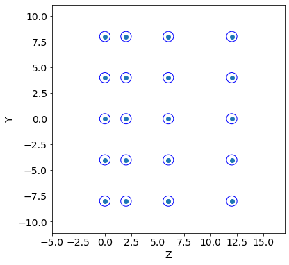
The module detector creates a simple 2D geometry of a wire based tracker made by 4 planes.

The adjustable parameters are the radius of each wire, the pitch (along the y axis), and the shift along y and z of a plane with respect to the previous one.

A total of 8 parameters can be tuned.

The goal of this toy model, is to tune the detector design so to optimize the efficiency (fraction of tracks which are detected) as well as the cost for its realization. As a proxy for the cost, we use the material/volume (the surface in 2D) of the detector. For a track to be detetected, in the efficiency definition we require at least two wires hit by the track.

So we want to maximize the efficiency (defined in detector.py) and minimize the cost.

LIST OF PARAMETERS

(baseline values)

• R = .5 [cm]

• pitch = 4.0 [cm]

• y1 = 0.0, y2 = 0.0, y3 = 0.0, z1 = 2.0, z2 = 4.0, z3 = 6.0 [cm]

# CONSTANT PARAMETERS
#------ define mother region ------#
y_min=-10.1
y_max=10.1
N_tracks = 1000


print("::::: BASELINE PARAMETERS :::::")
R = 0.5 #.5
pitch = 4.0 #10.0
y1 = 0.0
y2 = 0.0
y3 = 0.0
z1 = 2.0
z2 = 4.0
z3 = 6.0

print("R, pitch, y1, y2, y3, z1, z2, z3: ", R, pitch, y1, y2, y3, z1, z2, z3,"\n")


#------------- GEOMETRY ---------------#
print(":::: INITIAL GEOMETRY ::::")
tr = detector2.Tracker(R, pitch, y1, y2, y3, z1, z2, z3)
Z, Y = tr.create_geometry()
num_wires = detector2.calculate_wires(Y, y_min, y_max)


detector2.geometry_display(Z, Y, R, y_min=y_min, y_max=y_max,block=False,pause=5) #5

print("# of wires: ", num_wires)

#------------- TRACK GENERATION -----------#
print(":::: TRACK GENERATION ::::")
t = detector2.Tracks(b_min= y_min, b_max=y_max, alpha_mean=0, alpha_std=0.2) #b_min=-100, b_max=100
tracks = t.generate(N_tracks)

detector2.geometry_display(Z, Y, R, y_min=y_min, y_max=y_max,block=False, pause=-1)
detector2.tracks_display(tracks, Z,block=False,pause=-1)

 #a track is detected if at least two wires have been hit
score = detector2.get_score(Z, Y, tracks, R)
frac_detected = score[0]
print("fraction of tracks detected: ",frac_detected)

::::: BASELINE PARAMETERS :::::
R, pitch, y1, y2, y3, z1, z2, z3:  0.5 4.0 0.0 0.0 0.0 2.0 4.0 6.0 

:::: INITIAL GEOMETRY ::::
# of wires:  20
:::: TRACK GENERATION ::::

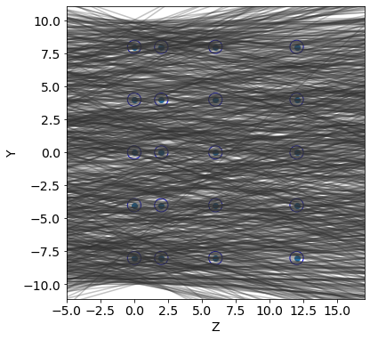
fraction of tracks detected:  0.264

---

Define Objectives

Defines the objective function of the problem that can be used in the Bayesian Optimization.

#------------- OBJECTIVE FUNCTION ---------------#

class Obj:

  def __init__(self,R=0.5,pitch=4.0):
    self.R = R
    self.pitch = pitch

  def update_pars(self,r,p):
    self.R = r
    self.pitch = p


  def objective(self,x):

    #you have to upack R, pitch if included in the BO
    y1, y2, y3, z1, z2, z3 = x
    Z, Y = detector2.Tracker(self.R, self.pitch, y1, y2, y3, z1, z2, z3).create_geometry()
    #a track is detected if at least two wires have been hit
    val = detector2.get_score(Z, Y, tracks, self.R)[0]
    #print(self.R, self.pitch)

    return 1. - val  # the smaller, the better.

---

Bayesian Optimization of the Detector Geometry

You can find different options for the optimization.

We refer to sklearn optimization package: https://scikit-optimize.github.io/stable/

Different approaches for the regression part.

from skopt import gp_minimize, gbrt_minimize, dummy_minimize

# You can change values within pre-defined ranges
# Below we are considering only the shifts along y and z
# (of each plane with respect to the previous plane)

y1_min, y1_max = [0., 4.]
y2_min, y2_max = [0., 4.]
y3_min, y3_max = [0., 4.]
z1_min, z1_max = [2., 10.]
z2_min, z2_max = [2., 10.]
z3_min, z3_max = [2., 10.]

dims = [(y1_min, y1_max),(y2_min, y2_max), (y3_min, y3_max),
        (z1_min, z1_max), (z2_min, z2_max),(z3_min, z3_max)]

ncalls = 100
rand_st = 1717 #for reproducibility

Bayesian Optimization with Gaussian Processes

obj_fun = Obj()

# https://scikit-optimize.github.io/stable/modules/generated/skopt.gp_minimize.html


res_gp = gp_minimize(
    func=obj_fun.objective,  # the function to minimize
    dimensions=dims,  # the bounds on each dimension of x
    acq_func="gp_hedge", #"gp_hedge",  # the acquisition function EI
    n_calls= ncalls,  # the number of evaluations of f
    n_random_starts=15,  # the number of random initialization points
    #noise=0.01**2,  # the noise level (optional)
    random_state=rand_st,  # the random seed, use same for reproducibility
    #kappa=kappa,  # the adjustable parameter of LCB; control variance
    #xi = xi, # adjustable parameter of either EI, PI: controls improvement
    verbose=False)

Results from BO(GP)

print("-------------------------------")
print("------RESULT FROM BO(GP)-------")
print("-------------------------------")

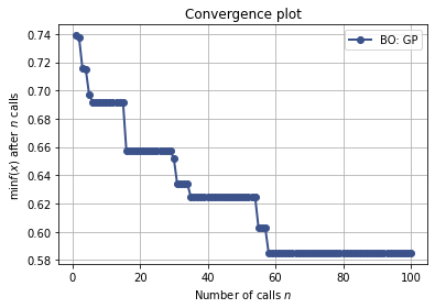
print("Objective optimum = ", res_gp.fun)
print("Best score (efficiency) = ", 1-res_gp.fun)

# get found optimal geometry #R, pitch,
[y1, y2, y3, z1, z2, z3] = res_gp.x

-------------------------------
------RESULT FROM BO(GP)-------
-------------------------------
Objective optimum =  0.585
Best score (efficiency) =  0.41500000000000004

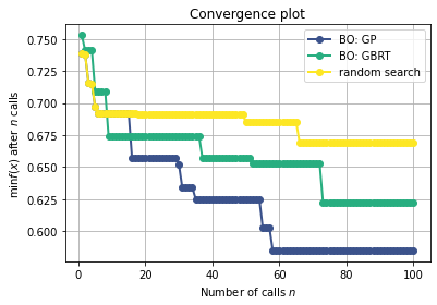
Convergence

print("....plotting convergence")
from skopt.plots import plot_convergence
plot_convergence(("BO: GP", res_gp))

....plotting convergence

<matplotlib.axes._subplots.AxesSubplot at 0x7f0de9cb0c90>

Optimal Geometry

#------------- GEOMETRY ---------------#
print(":::: OPTIMAL GEOMETRY ::::")

tr = detector2.Tracker(R, pitch, y1, y2, y3, z1, z2, z3)
Z, Y = tr.create_geometry()
num_wires = detector2.calculate_wires(Y, y_min, y_max)
print("num_wires: ", num_wires)

detector2.geometry_display(Z, Y, R, y_min=y_min, y_max=y_max,block=False, pause=-1)
detector2.tracks_display(tracks, Z,block=False,pause=-1)

#a track is detected if at least two wires have been hit
score = detector2.get_score(Z, Y, tracks, R)
frac_detected = score[0]
print("fraction of tracks detected: ",frac_detected)

:::: OPTIMAL GEOMETRY ::::
num_wires:  20

fraction of tracks detected:  0.415

Bayesian Optimization with GBRT

res_gbrt = gbrt_minimize(
    func=obj_fun.objective,  # the function to minimize
    dimensions=dims,  # the bounds on each dimension of x
    acq_func="EI",  # the acquisition function EI
    n_calls= ncalls,  # the number of evaluations of f
    n_random_starts=15,  # the number of random initialization points
    random_state=rand_st,  # the random seed, use same for reproducibility
    #kappa=kappa,  # the adjustable parameter of LCB; control variance
    #xi = xi, # adjustable parameter of either EI, PI: controls improvement
    verbose=False)

print("-------------------------------")
print("-----RESULT FROM BO(GBRT)------")
print("-------------------------------")

print("Objective optimum = ", res_gbrt.fun)
print("Best score = ", 1-res_gbrt.fun)

-------------------------------
-----RESULT FROM BO(GBRT)------
-------------------------------
Objective optimum =  0.622
Best score =  0.378

Random Search

res_rand = dummy_minimize(
    func=obj_fun.objective,  # the function to minimize
    dimensions=dims,  # the bounds on each dimension of x
    n_calls= ncalls,  # the number of evaluations of f
    random_state=rand_st,  # the random seed
    verbose=False)

print("-------------------------------")
print("------  RESULT FROM RS  -------")
print("-------------------------------")

print("Objective optimum = ", res_rand.fun)
print("Best score = ", 1-res_rand.fun)

-------------------------------
------  RESULT FROM RS  -------
-------------------------------
Objective optimum =  0.669
Best score =  0.33099999999999996

Visualization of Results

print("....plotting convergence")
from skopt.plots import plot_convergence
plot_convergence(("BO: GP", res_gp),("BO: GBRT", res_gbrt),("random search", res_rand))

....plotting convergence

<matplotlib.axes._subplots.AxesSubplot at 0x7f0dc912c550>

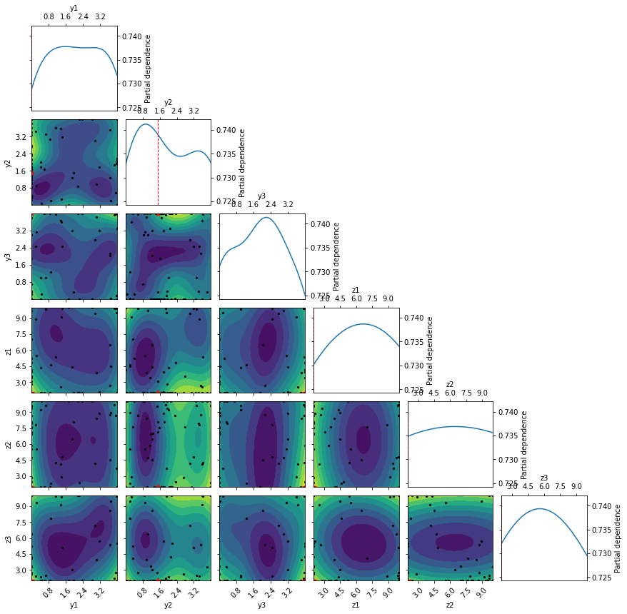
list_str = ["y1", "y2", "y3", "z1", "z2", "z3"] #----"R", "pitch"

from skopt.plots import plot_objective
_ = plot_objective(res_gp,dimensions=list_str)

---

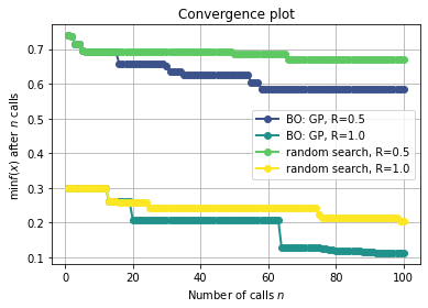
Solution 1

1. Increase radius to 1.0 and compare convergence plots of GP and RS with before.

R, pitch = 1.0, 4.0 #to update final plot of optimal geometry

obj_fun.update_pars(R, pitch)

res_gp_largeR = gp_minimize(
    func=obj_fun.objective,  # the function to minimize
    dimensions=dims,  # the bounds on each dimension of x
    acq_func="gp_hedge", #"gp_hedge",  # the acquisition function EI
    n_calls= ncalls,  # the number of evaluations of f
    n_random_starts=15,  # the number of random initialization points
    random_state=rand_st,  # the random seed, use same for reproducibility
    verbose=False)

print("-------------------------------")
print("------  RESULT FROM GP  -------")
print("-------------------------------")

print("Objective optimum = ", res_gp_largeR.fun)
print("Best score = ", 1-res_gp_largeR.fun)

-------------------------------
------  RESULT FROM GP  -------
-------------------------------
Objective optimum =  0.11299999999999999
Best score =  0.887

res_rand_largeR = dummy_minimize(
    func=obj_fun.objective,  # the function to minimize
    dimensions=dims,  # the bounds on each dimension of x
    n_calls= ncalls,  # the number of evaluations of f
    random_state=rand_st,  # the random seed
    verbose=False)

print("-------------------------------")
print("------  RESULT FROM RS  -------")
print("-------------------------------")

print("Objective optimum = ", res_rand_largeR.fun)
print("Best score = ", 1-res_rand_largeR.fun)

-------------------------------
------  RESULT FROM RS  -------
-------------------------------
Objective optimum =  0.20399999999999996
Best score =  0.796

print("....plotting convergence")
from skopt.plots import plot_convergence
plot_convergence(("BO: GP, R=0.5", res_gp),("BO: GP, R=1.0", res_gp_largeR),("random search, R=0.5", res_rand),("random search, R=1.0", res_rand_largeR))

....plotting convergence

<matplotlib.axes._subplots.AxesSubplot at 0x7f0de9b1bd10>

print(res_gp_largeR.fun)
print(res_gp.fun)

0.11299999999999999
0.585

[y1, y2, y3, z1, z2, z3] = res_gp_largeR.x

#------------- GEOMETRY ---------------#
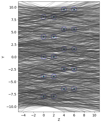
print(":::: OPTIMAL GEOMETRY ::::")

tr = detector2.Tracker(R, pitch, y1, y2, y3, z1, z2, z3)
Z, Y = tr.create_geometry()
num_wires = detector2.calculate_wires(Y, y_min, y_max)
print("num_wires: ", num_wires)

detector2.geometry_display(Z, Y, R, y_min=y_min, y_max=y_max,block=False, pause=-1)
detector2.tracks_display(tracks, Z,block=False,pause=-1)

#a track is detected if at least two wires have been hit
score = detector2.get_score(Z, Y, tracks, R)
frac_detected = score[0]
print("fraction of tracks detected: ",frac_detected)

:::: OPTIMAL GEOMETRY ::::
num_wires:  21

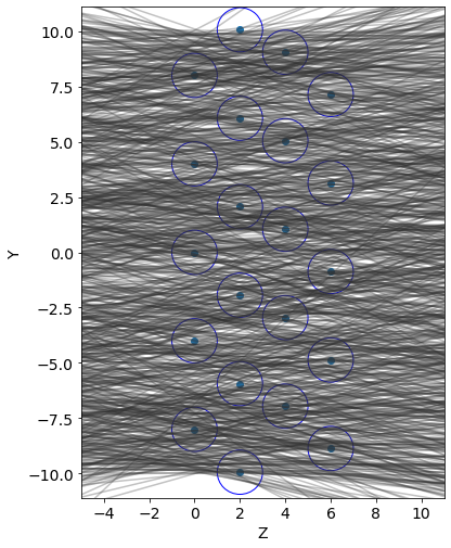
fraction of tracks detected:  0.887