Regularization and Cross-Validations

When Linear Regression Fails

In this context fails means that OLS is unable to provide a unique solution, such as a unique set of coefficients for the input variables.

Plain vanilla multiple linear regression (OLS) fails if the number of observations is smaller than the number of features.

Example: If the dependent variable is the Sales Price, we cannot uniquely determine the weights for the features if we have only 4 observations.

Dist. to School	Prop. Area	Housing Area	Value	Prop. Tax	Bathrooms	Sales Price
7	0.4	1800	234	9.8	2	267.5
2.3	0.8	1980	244	10.5	2.5	278.2
4.3	1.1	2120	252	16.2	3	284.5
3.8	0.6	2500	280	18.4	3.5	310.4

Suppose we want to predict the “Sales Price” by using a linear combination of the feature variables, such as “Distance to School”, “Property Area”, etc.

\[\large M\cdot \vec{\beta} = \beta_1\cdot col_1(M)+\beta_2\cdot col_2(M)+...+\beta_p\cdot col_p(M)\]

The Ordinary Least Squares (OLS) method aims at finding the coefficients \(\beta\) such that the the sum or squared errors is minimal, i.e.

\[\large \underset{\beta}{\operatorname{argmin}}\|\text{Sales Price}- M\cdot \vec{\beta}\|^2\]

Important Question: Why does OLS fail in this case? Hint: the problem to solve is ill-posed, in the sense that it allows many perfect solutions.

What does Rank Deficiency mean, and why we need Regularization?

The assumption for multiple linear regression is

\[\large Y = X\beta + \sigma \epsilon \]

where \(\sigma\) is the standard deviatin of the noise. Further, we assume that the “noise” \(\epsilon\) is independent and identically distributed with a zero mean.

We believe that the output is a linear combination of the input features.

Thus, if we would like to solve for the “weights” \(\beta\) we may consider

\[\large X^tY = X^tX\beta+\sigma X^t\epsilon \]

And if the matrix \(X^tX\) is invertible then we can solve for expected value of \(\beta\):

\[\large \mathbb{E}(\beta) = (X^tX)^{-1}X^t Y \]

We can show by using Linear Algebra that the OLS solution obtained form minimizing the sum of the square residuals is equivalent.

We can test whether the matrix \(X^tX\) is invertible by simply computing its determinant and checking that it is not zero.

IMPORTANT: When the matrix \(X^tX\) is not invertible we cannot apply this method to get \(\mathbb{E}(\beta)\). In this case if we minimize the sum of the squared residuals the algorithm cannot find just one best solution.

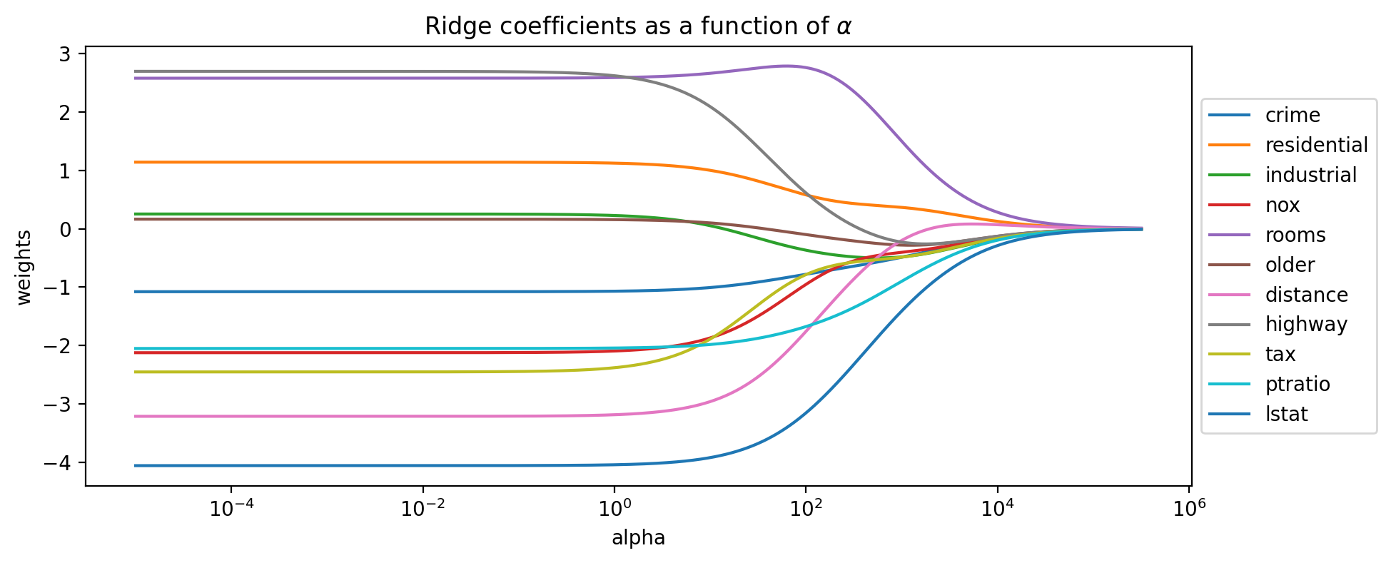
A solution for rank defficient Multiple Linear Regression: L2 (Ridge) Regularization

Main Idea: minimize the sum of the square residuals plus a constraint on the vector of weights

The L2 norm is

\[ \|\beta\|_2:=\left(\sum_{j=1}^{p}\beta_j^2\right)^{1/2} \]

The Ridge model (also known as the Tikhonov regularization) consists of learning the weights by the following optimization:

\[\text{minimize} \frac{1}{n}\sum_{i=1}^{n}\left(\text{Residual}_i\right)^2 + \alpha \sum\limits_{j=1}^{p}\beta_j^2\]

where \(\alpha\) is a constant that can be adjusted based on a feedback loop so it is a hyperparameter (“tunning” parameter).

This optimization is equivalent to minimizing the sum of the square residuals with a constraint on the sum of the squared weights

\[\text{minimize} \frac{1}{n}\sum_{i=1}^{n}\left(\text{Residual}_i\right)^2\]

subject to

\[ \sum\limits_{j=1}^{p}\beta_j^2 < M \]

Important: What happens with the solution \(\beta\) when the hyperparameter \(\alpha\) grows arbitrarily large? Hint: generate a mapping and plot the coefficient paths.

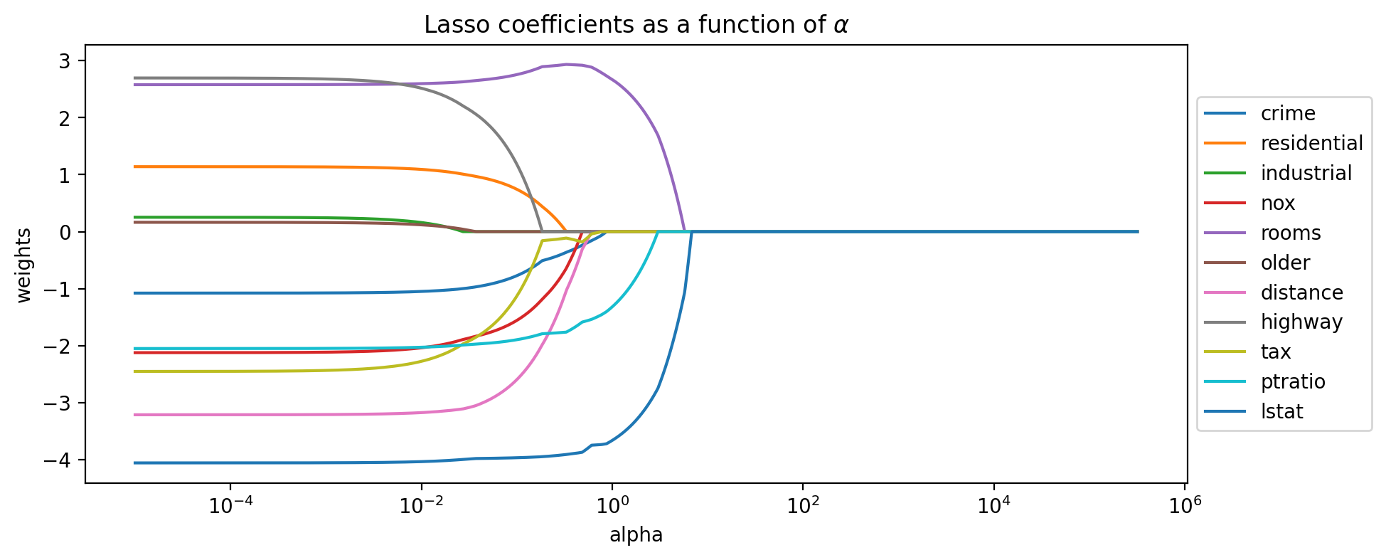
L1 (Lasso) Regularization

The L1 norm is

\[ \|\beta\|_1:=\sum_{j=1}^{p}|\beta_j| \]

The Lasso model consists of learning the weights by the following optimization:

\[\text{minimize} \frac{1}{n}\sum_{i=1}^{n}\left(\text{Residual}_i\right)^2 + \alpha \|\beta\|_1\]

where \(alpha\) is a constant that can be adjusted based on a feedback loop so it is a hyperparameter.

This optimization is equivalent to minimizing the sum of the square residuals with a constraint on the sum of the squared weights

\[\text{minimize} \frac{1}{n}\sum_{i=1}^{n}\left(\text{Residual}_i\right)^2\]

subject to

\[ \sum\limits_{j=1}^{p}|\beta_j| < M \]

The difference between L1 and L2 norms

In the following example the L2 norm of the vector \(\vec{AB}\) is 5 and the L1 norm is \(4+3=7\).

The difference between the L1 and L2 norms

Geometric comparison in 2D between L1 and L2 norms

Difference between L1 and L2

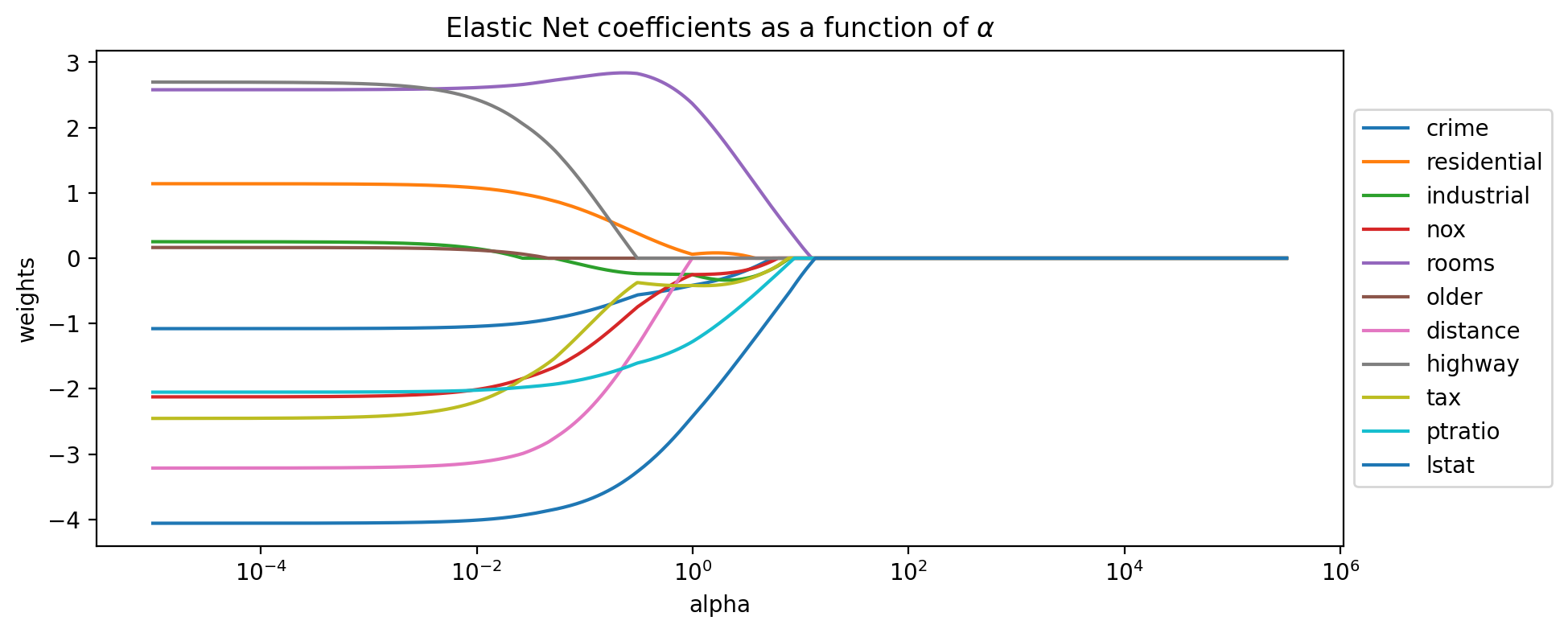
Elastic Net Regularization

Tha main idea is to combine the L2 and L1 regularizations in a weighted way, such as:

\[ \lambda\cdot \sum\limits_{j=1}^{p}|\beta_j| + 0.5\cdot (1-\lambda)\cdot\sum\limits_{j=1}^{p}\beta_j^2 \]

Here \(0\leq\lambda\leq1\) is called the L1_ratio.

The Elstic Net regularization consists of learning the weights by solving the following optimization problem:

\[\text{minimize} \frac{1}{n}\sum_{i=1}^{n}\left(\text{Residual}_i\right)^2 + \alpha\left( \lambda\cdot \sum\limits_{j=1}^{p}|\beta_j| + 0.5\cdot (1-\lambda)\cdot\sum\limits_{j=1}^{p}\beta_j^2\right)\]

So with this rgularization approach we have two hyperparameters that we need to decide on.

Model Validation via k-Fold Cross-Validations

In general: how do we know that the predictions made are good?

For many applications you can think of a data set representing both “present” and “future.”

In order to compare the predictive power of different models we use K-fold cross-validation.

How do we get unbiased estimates of errors?

Example schematic of 5-fold cross-validation:

Step 1 in the 5-fold cross-validation

Coding Applications

---

Setup

import os
if 'google.colab' in str(get_ipython()):
  print('Running on CoLab')
  from google.colab import drive
  drive.mount('/content/drive')
  os.chdir('/content/drive/My Drive/Data Sets')
  !pip install -q pygam
else:
  print('Running locally')
  os.chdir('../Data')

%matplotlib inline
%config InlineBackend.figure_format = 'retina'
import numpy as np
import matplotlib.pyplot as plt
import pandas as pd
import statsmodels.api as sm
from sklearn.model_selection import RepeatedKFold
from sklearn.model_selection import KFold
from sklearn.model_selection import train_test_split as tts
from sklearn.metrics import mean_squared_error as mse
from sklearn.preprocessing import StandardScaler
from sklearn.model_selection import cross_val_score

from sklearn.linear_model import ElasticNet, Ridge, Lasso

Data Import

data_housing = pd.read_csv('../Data/housing.csv')
data_concrete = pd.read_csv('../Data/concrete.csv')

Coefficient Paths

feats = ['crime','residential','industrial','nox','rooms','older','distance','highway','tax','ptratio','lstat']
X = data_housing[feats]
y = data_housing['cmedv'].values

scale = StandardScaler()
Xs = scale.fit_transform(X)

# generate the coefficients for Ridge regression and many values of alpha
n_alphas = 2000
alphas = np.logspace(-5, 5.5, n_alphas)

coefs = []
for a in alphas:
    ridge = Ridge(alpha=a, fit_intercept=False)
    ridge.fit(Xs, y)
    coefs.append(ridge.coef_)

# Display coefficient paths Ridge
plt.figure(figsize=(10, 4))

ax = plt.gca()
ax.plot(alphas, coefs)
ax.set_xscale('log')
plt.xlabel('alpha')
plt.ylabel('weights')
plt.title('Ridge coefficients as a function of $\\alpha$')
plt.axis('tight')
plt.legend(feats, bbox_to_anchor=[1,0.5], loc='center left')
plt.show()

# generate the coefficients for Ridge regression and many values of alpha
n_alphas = 2000
alphas = np.logspace(-5, 5.5, n_alphas)

coefs = []
for a in alphas:
    model = Lasso(alpha=a, fit_intercept=False)
    model.fit(Xs, y)
    coefs.append(model.coef_)

# Display coefficient paths Ridge
plt.figure(figsize=(10, 4))

ax = plt.gca()
ax.plot(alphas, coefs)
ax.set_xscale('log')
plt.xlabel('alpha')
plt.ylabel('weights')
plt.title('Lasso coefficients as a function of $\\alpha$')
plt.axis('tight')
plt.legend(feats, bbox_to_anchor=[1,0.5], loc='center left')
plt.show()

# generate the coefficients for Ridge regression and many values of alpha
n_alphas = 2000
alphas = np.logspace(-5, 5.5, n_alphas)

coefs = []
for a in alphas:
    model = ElasticNet(alpha=a, fit_intercept=False)
    model.fit(Xs, y)
    coefs.append(model.coef_)# generate the coefficients for Ridge regression and many values of alpha
n_alphas = 2000
alphas = np.logspace(-5, 6, n_alphas)

coefs = []
for a in alphas:
    ridge = Ridge(alpha=a, fit_intercept=False)
    ridge.fit(Xs, y)
    coefs.append(ridge.coef_)

# Display coefficient paths Ridge
plt.figure(figsize=(10, 4))

ax = plt.gca()
ax.plot(alphas, coefs)
ax.set_xscale('log')
plt.xlabel('alpha')
plt.ylabel('weights')
plt.title('Elastic Net coefficients as a function of $\\alpha$')
plt.axis('tight')
plt.legend(feats, bbox_to_anchor=[1,0.5], loc='center left')
plt.show()