Supervised Learning - Decision Trees, Random Forest and eXtreme Gradient Boosting (XGBoost)

What is a Decision Tree?

• Main Idea: organize the feature space in as a collection of units (in Euclidean space, rectangular boxes) such that all observations in each unit have some homogeneity (similar range of one or more features). As such, every observation goes into some unit and the predicted value is assigned by computing the mean (regression) or the votes (classification) over the entire unit.

• General View: the input features can be a mix of discrete and continuous variables and the dependent variable can be either continuous (for regression problems) or discrete (for classification problems).

• Important: This is an iterative process. The decisions are nodes in the tree, from each node we split two branches. The decisions are informed by objective functions (e.g. we can think of mean squared error for regression or the Gini impurity for classification). The final decisions are represented as piecewise defined, step functions.

Example: predict the mileage of the car by using its weight in 1000 lbs. (MTCars data set).

MPG prediction based on the weight of the car.

The following is a visualization in the feature-vs-target space:

MPG prediction based on the weight of the car.

Example: predict the mileage of the car by using weight and HP. (MTCars data set).

MPG prediction based on the weight of the car.

In a two-dimensional feature space, below we have a visualization example of the compartmentalization by decision trees:

Visualization of the step function created with decision trees.

Decision Trees for Regression

Measuring Loss: for the objective function we can use either the mean absolute error or the mean square error.

Algorithm:

Decision Trees for Classification

Example: A biologist recorded the weights of rabbits and squirrels in a data set. A decision tree starts with the root node such as if the weight is less than a threshold value, then inside the resulting subset (branch) there are more squirrels than rabbits.

Measuring Loss: The Gini impurity index measures the likelihood of missclassification in each node:

\[\large G:= \sum_{i=1}^{C} p(i)\cdot(1-p(i))= 1 - \sum_{i=1}^{C} p^2(i)\]

where \(C\) is the number of distinct classes and \(p(i)\) represents the probability of choosing and element of class \(i\) if one individual is randomly selected in the node.

Example of a Decision Tree for Classification.

For a binary classification problem, we can think of approximating two distinct probability distributions:

Separating different distributions.

Random Forests

Original Abstract (L. Breiman, 2001): Random forests are a combination of tree predictors such that each tree depends on the values of a random vector sampled independently and with the same distribution for all trees in the forest. The generalization error for forests converges almost surely to a limit as the number of trees in the forest becomes large. The generalization error of a forest of tree classifiers depends on the strength of the individual trees in the forest and the correlation between them. Using a random selection of features to split each node yields error rates that compare favorably to Adaboost (Freund and Schapire[1996]), but are more robust with respect to noise. Internal estimates monitor error, strength, and correlation and these are used to show the response to increasing the number of features used in the splitting. Internal estimates are also used to measure variable importance. These ideas are also applicable to regression.

Main Idea: grow many decision trees based on random samples of set of observations and then average the predictions across the trees in the forest for the final answer. One important aspect is that the random sampling is done with replacement (“bootstrap aggregation”).

Decision Boundaries Comparison

An example of decision boundaries for Decsion Trees vs Random Forest.

Boosting

Boosting (Schapire and Freund 2012) is a greedy algorithm for fitting adaptive basis-function where the weights are generated by an algorithm called a weak learner or a base learner. The algorithm works by applying the weak learner sequentially to weighted versions of the data, where more weight is given to examples that were misclassified by earlier rounds. This weak learner can be any classification or regression algorithm. In 1998, the late Leo Breiman called boosting, where the weak learner is a shallow decision tree, the “best off-the-shelf classifier in the world” (Hastie et al. 2009, p340). (Reference: K. Murphy - “Machine Learning - A Probilistic Perspective”, page 554.)

How Does Adaptive Boosting Work?

We can understand the working of the AdaBoost algorithm in step by step manner as going deep into the work, we can see there are multiple basic steps which this algorithm follows. Let’s take a look at these steps.

1. When the algorithm is given data, it starts by assigning equal weights to all training examples in the dataset. These weights represent the importance of each sample during the training process.

2. Here, this algorithm iterates with a few algorithms for a specified number of iterations (or until a stopping criterion is met). The algorithm trains a weak classifier on the training data. Here the weak classifier can be considered a model that performs slightly better than random guessing, such as a decision stump (a one-level decision tree).

3. During each iteration, the algorithm trains the weak classifier on given training data with the current sample weights. The weak classifier aims to minimize the classification error, weighted by the sample weights.

4. After training the weak classifier, the algorithm calculates classifier weight based on the errors of the weak classifier. A weak classifier with a lower error receives a higher weight.

5. Once the calculation of weight completes, the algorithm updates sample weights, and the algorithm gives assigns higher weights to misclassified examples so that more importance in subsequent iterations can be given.

6. After updating the sample weights, they are normalized so that they sum up to 1 and Combine the predictions of all weak classifiers using a weighted majority vote. The weights of the weak classifiers are considered when making the final prediction.

7. Finally, Steps 2–5 are repeated for the specified number of iterations (or until the stopping criterion is met), with the sample weights updated at each iteration. The final prediction is obtained by aggregating the predictions of all weak classifiers based on their weights.

The below pseudocode can be helpful in understanding the working of the AdaBoost algorithm.

Initialize sample weights for each training example
For each iteration:
- Train a weak classifier using the current sample weights
- Calculate the error of the weak classifier
- Calculate the weight of the weak classifier based on the error
- Update the sample weights based on the weak classifier's performance
- Normalize the sample weights
End the iterations
Combine the weak classifiers using a weighted majority vote.

Reference: https://medium.com/@datasciencewizards/understanding-the-adaboost-algorithm-2e9344d83d9b

Gradient Boosting

Assume you have an regressor \(F\) and, for the observation \(x_i\) we make the prediction \(F(x_i)\). To improve the predictions, we can regard \(F\) as a ‘weak learner’ and therefore train a decision tree (we can call it \(h\)) where the new output is \(y_i-F(x_i)\). So, the new predictor is trained on the residuals of the previous one. Thus, there are increased chances that the new regressor

\[\large F + h\]

is better than the old one, \(F.\)

Main task: implement this idea in an algorithm and test it on real data sets.

Gradient Boosting w/Two Steps for Regression

eXtreme Gradient Boosting (XGBoost)

XGBoost is a powerful and widely used machine learning algorithm. It’s a specific implementation of gradient boosting, a technique that builds an ensemble of predictive models (typically decision trees) in a sequential manner. Each new model focuses on correcting the errors of the previous ones, leading to a final model that is often significantly more accurate than any of its individual components.

How Does XGBoost Work?

• Initialization: XGBoost begins by creating a simple initial model, usually a single decision tree, that makes predictions based on the input features. This initial model will likely have errors.

• Gradient Calculation: XGBoost then calculates the gradients of the loss function (a measure of how well the model is performing) with respect to the predictions of the current model. These gradients indicate the direction and magnitude of changes needed to improve the predictions.

• New Tree Creation: A new decision tree is trained to predict these gradients. This tree essentially learns how to correct the errors of the previous model.

• Tree Weighting: The new tree is added to the ensemble with a weight that determines how much influence it has on the final predictions. This weight is typically a small value to avoid overfitting.

• Iteration: Steps 2-4 are repeated for a specified number of iterations or until the model’s performance stops improving. With each iteration, new trees are added to the ensemble, each focusing on correcting the residual errors of the previous trees.

• Final Prediction: The final prediction is made by summing the weighted predictions of all the trees in the ensemble.

Key Features and Advantages of XGBoost:

• Regularization: XGBoost includes regularization techniques (L1 and L2 regularization) to prevent overfitting, making it more robust to noise and outliers in the data.

• Handling Missing Values: XGBoost can automatically handle missing values in the input data without requiring explicit imputation.

• Parallelization: The algorithm can be parallelized across multiple cores or machines, making it scalable to large datasets.

• Tree Pruning: XGBoost prunes trees during training to remove branches that don’t contribute significantly to the model’s accuracy, further preventing overfitting.

• Feature Importance: It provides a measure of feature importance, allowing you to understand which features are most influential in making predictions. Where is XGBoost Used?

XGBoost is extremely versatile and is used in a wide range of applications, including:

• Classification: Predicting categorical outcomes (e.g., customer churn, fraud detection, disease diagnosis) Regression: Predicting continuous outcomes (e.g., house prices, stock prices, sales forecasting) Ranking: Ranking items in order of relevance (e.g., search engine results, product recommendations) Important Considerations:

XGBoost can be sensitive to hyperparameter tuning, so careful optimization is often required. It may be computationally expensive for very large datasets.

Code Applications

---

Setup

import os
if 'google.colab' in str(get_ipython()):
  print('Running on CoLab')
  from google.colab import drive
  drive.mount('/content/drive')
  os.chdir('/content/drive/My Drive/Data Sets')
  !pip install -q pygam
  !pip install -q dtreeviz
else:
  print('Running locally')
  os.chdir('../Data')

Running on CoLab
Drive already mounted at /content/drive; to attempt to forcibly remount, call drive.mount("/content/drive", force_remount=True).
     ━━━━━━━━━━━━━━━━━━━━━━━━━━━━━━━━━━━━━━━━ 91.8/91.8 kB 1.6 MB/s eta 0:00:00
?25h

# import libraries
import numpy as np
import pandas as pd
import pydot
from IPython.display import Image

from xgboost import XGBClassifier

%matplotlib inline
%config InlineBackend.figure_format = 'retina'
import matplotlib.pyplot as plt
from matplotlib.colors import ListedColormap
import seaborn as sns

from sklearn.preprocessing import MinMaxScaler
from sklearn.model_selection import StratifiedKFold, cross_val_score
from sklearn.metrics import accuracy_score
from sklearn import tree
import dtreeviz

Data import

data_example_1 = pd.read_csv('example_data_classification.csv', header=None)
data_fusion_experiment = pd.read_csv('fusion_experiment.csv')

Example 1

data_example_1.columns = ['Exam 1','Exam 2','Status']

data_example_1

	Exam 1	Exam 2	Status
0	34.623660	78.024693	0
1	30.286711	43.894998	0
2	35.847409	72.902198	0
3	60.182599	86.308552	1
4	79.032736	75.344376	1
...	...	...	...
95	83.489163	48.380286	1
96	42.261701	87.103851	1
97	99.315009	68.775409	1
98	55.340018	64.931938	1
99	74.775893	89.529813	1

100 rows × 3 columns

x = data_example_1[['Exam 1','Exam 2']]
y = data_example_1['Status']

model = tree.DecisionTreeClassifier(max_depth=4,min_samples_leaf=5,random_state=123)
model.fit(x,y)

DecisionTreeClassifier(max_depth=4, min_samples_leaf=5, random_state=123)

In a Jupyter environment, please rerun this cell to show the HTML representation or trust the notebook.
On GitHub, the HTML representation is unable to render, please try loading this page with nbviewer.org.

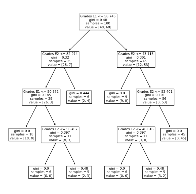
plt.figure(figsize=(8,8))
tree.plot_tree(model,feature_names = ['Grades E1','Grades E2'])
plt.savefig('DecisionTree_Example.svg', bbox_inches='tight')
plt.show()

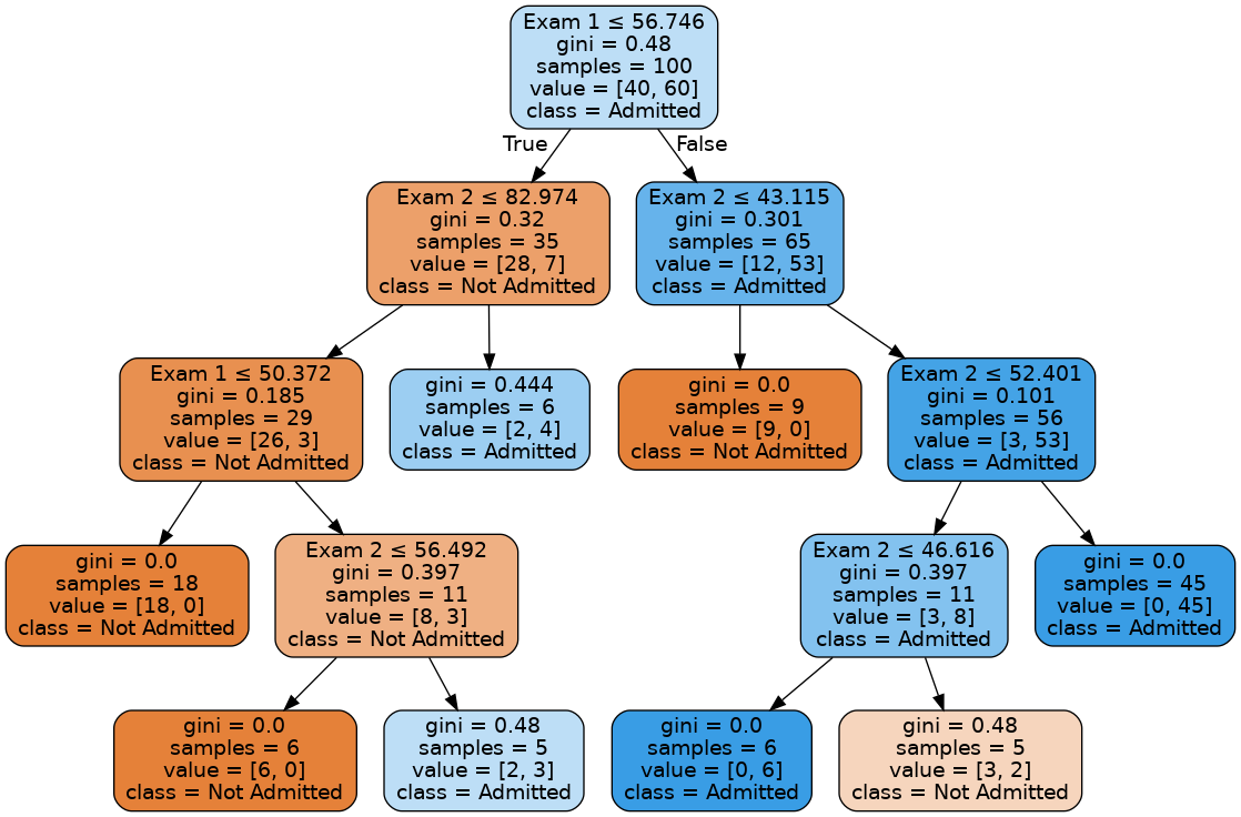
def ShowTree(classifier, features, classes):
    dot_data = tree.export_graphviz(model, out_file=None, filled=True, rounded=True,
                special_characters=True, feature_names=x.columns, class_names=classes)
    (g,) = pydot.graph_from_dot_data(dot_data)
    #g.set_dpi('100')
    g.write_png('tree.png')
    return Image(g.create_png())

ShowTree(model, x.columns,['Not Admitted','Admitted'])

h = .1 # step size in the grid of points
cmap_light = ListedColormap(['#FFD0D7', 'lightcyan'])
cmap_bold = ListedColormap(['red', 'navy'])

# create a grid of values for the features' space
x_min, x_max = x.values[:, 0].min() - 1, x.values[:, 0].max() + 1
y_min, y_max = x.values[:, 1].min() - 1, x.values[:, 1].max() + 1
xx, yy = np.meshgrid(np.arange(x_min, x_max, h),
                         np.arange(y_min, y_max, h))

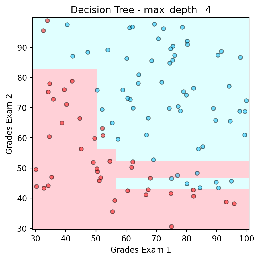
Example of Decision Boundary from a Binary Tree

# filter out the applicants that got admitted
admitted = data_example_1.loc[y == 1]

# filter out the applicants that din't get admission
not_admitted = data_example_1.loc[y == 0]


# show the decision boundary in the features' space
Z = model.predict(pd.DataFrame(np.c_[xx.ravel(), yy.ravel()],columns=['Exam 1','Exam 2']))

# Put the result into a color plot
Z = Z.reshape(xx.shape)
fig, ax = plt.subplots()
plt.pcolormesh(xx, yy, Z, cmap=cmap_light)


# Plot also the points
plt.scatter(admitted.iloc[:, 0], admitted.iloc[:, 1], color ='deepskyblue', s=25, label='Admitted',ec='k',alpha=0.5)
plt.scatter(not_admitted.iloc[:, 0] ,not_admitted.iloc[:, 1], color ='red', s=25,ec='k',alpha=0.5, label='Not Admitted')
plt.xlim(xx.min(), xx.max())
plt.xlabel('Grades Exam 1')
plt.ylabel('Grades Exam 2')
plt.ylim(yy.min(), yy.max())
ax.set_aspect('equal', 'box')
plt.title("Decision Tree - max_depth=4")
print('Accuracy : ' + str(accuracy_score(y,model.predict(x))))
plt.savefig('dtree.png',dpi=300)
plt.show()

Accuracy : 0.94

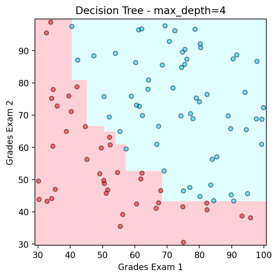
Example of Decision Boundary from XGBoost

model = XGBClassifier(n_estimators=10, max_depth = 4,random_state=123)
model.fit(x,y)

XGBClassifier(base_score=None, booster=None, callbacks=None,
              colsample_bylevel=None, colsample_bynode=None,
              colsample_bytree=None, device=None, early_stopping_rounds=None,
              enable_categorical=False, eval_metric=None, feature_types=None,
              gamma=None, grow_policy=None, importance_type=None,
              interaction_constraints=None, learning_rate=None, max_bin=None,
              max_cat_threshold=None, max_cat_to_onehot=None,
              max_delta_step=None, max_depth=4, max_leaves=None,
              min_child_weight=None, missing=nan, monotone_constraints=None,
              multi_strategy=None, n_estimators=10, n_jobs=None,
              num_parallel_tree=None, random_state=123, ...)

In a Jupyter environment, please rerun this cell to show the HTML representation or trust the notebook.
On GitHub, the HTML representation is unable to render, please try loading this page with nbviewer.org.

# show the decision boundary in the features' space
Z = model.predict(pd.DataFrame(np.c_[xx.ravel(), yy.ravel()],columns=['Exam 1','Exam 2']))

# Put the result into a color plot
Z = Z.reshape(xx.shape)
fig, ax = plt.subplots()
plt.pcolormesh(xx, yy, Z, cmap=cmap_light)


# Plot also the points
plt.scatter(admitted.iloc[:, 0], admitted.iloc[:, 1], color ='deepskyblue', s=25, label='Admitted',ec='k',alpha=0.5)
plt.scatter(not_admitted.iloc[:, 0] ,not_admitted.iloc[:, 1], color ='red', s=25,ec='k',alpha=0.5, label='Not Admitted')
plt.xlim(xx.min(), xx.max())
plt.xlabel('Grades Exam 1')
plt.ylabel('Grades Exam 2')
plt.ylim(yy.min(), yy.max())
ax.set_aspect('equal', 'box')
plt.title("Decision Tree - max_depth=4")
print('Accuracy : ' + str(accuracy_score(y,model.predict(x))))
plt.savefig('dtree.png',dpi=300)
plt.show()

Accuracy : 1.0

Example 2 - Fusion Experiment Data

data_fusion_experiment.drop(columns=['Unnamed: 0'],inplace=True)

data_fusion_experiment

	Magnetic Field Fluctuations	Leakage	Instabilities	Plasma Instabilities	Magnetic Field Strength	Magnetic Field Configuration	Injection Energy	Beam Symmetry	Target Density	Target Composition	Fuel Density	Temperature	Confinement Time	Fuel Purity	Energy Input	Power Output	Pressure	Neutron Yield	Ignition
0	0.037454	0.058078	0.028259	0.015705	9.000578	tokamak	5.713125	0.800007	2.026963e+19	deuterium	7.612226e+19	4.050388e+08	0.842126	99.971295	250.726719	55.321517	6.107792e+06	5.443404e+10	0
1	0.095071	0.052697	0.045868	0.009551	3.841421	reversed field pinch	9.819548	0.082642	3.050685e+19	deuterium-tritium	8.742441e+19	2.551963e+08	0.504637	99.951049	345.614166	22.767959	4.921946e+06	8.372016e+10	0
2	0.073199	0.035104	0.009922	0.013794	1.467187	stellarator	7.016781	0.176319	5.287388e+19	tritium	8.236610e+19	2.627651e+08	0.357445	99.958831	290.050980	49.872944	9.798230e+06	8.112584e+10	1
3	0.059866	0.049321	0.044684	0.047349	9.277696	tokamak	4.018930	0.833709	5.961305e+19	deuterium-tritium	9.079654e+19	3.104709e+08	0.992195	99.997186	436.491093	2.656182	5.611293e+06	4.423307e+10	1
4	0.015602	0.036510	0.020308	0.088453	4.926347	reversed field pinch	6.145836	0.808161	7.887942e+19	deuterium	8.186142e+19	3.258529e+08	0.648677	99.927054	198.773196	48.096005	8.541064e+06	2.245276e+10	0
...	...	...	...	...	...	...	...	...	...	...	...	...	...	...	...	...	...	...	...
99995	0.079230	0.062215	0.009281	0.075015	6.989681	tokamak	8.363230	0.080241	6.220430e+19	deuterium-tritium	8.029543e+19	3.534515e+08	0.434566	99.917577	130.728901	51.822726	9.611845e+06	6.252602e+10	0
99996	0.077925	0.062922	0.062563	0.027253	9.904975	reversed field pinch	3.718771	0.977716	3.429971e+19	tritium	1.608651e+19	4.554238e+08	0.888713	99.902695	114.869008	9.746068	1.099463e+06	4.545773e+10	0
99997	0.067445	0.019220	0.062666	0.057559	5.389669	tokamak	8.788397	0.374680	4.750184e+19	tritium	3.021016e+19	2.331046e+08	0.323766	99.910285	458.044080	69.116870	7.473165e+06	7.240109e+10	0
99998	0.049945	0.065308	0.004765	0.089334	6.984881	tokamak	3.024949	0.926179	3.030606e+19	deuterium-tritium	4.217068e+19	2.660837e+08	0.646530	99.984932	342.844863	31.591851	6.759779e+06	7.576517e+10	0
99999	0.038991	0.000156	0.070408	0.050242	6.640008	tokamak	6.296842	0.885714	7.313929e+19	deuterium	3.560199e+19	4.370338e+08	0.982118	99.978973	478.135341	92.487755	5.169346e+06	9.004981e+10	0

100000 rows × 19 columns

r=4
c=5
it=1
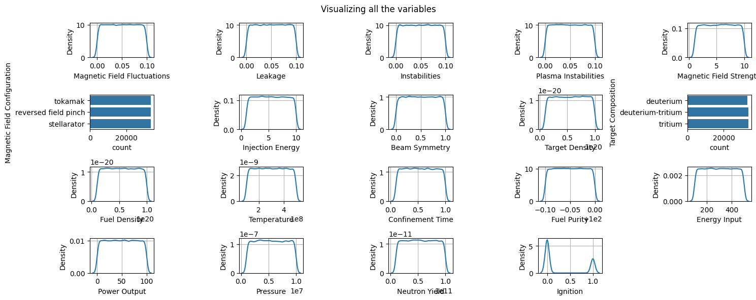
plt.figure(figsize=(15,6))
for i,j in enumerate(data_fusion_experiment.columns):
    plt.suptitle("Visualizing all the variables")
    plt.subplot(r,c,it)
    if data_fusion_experiment[j].dtype=='object':
        sns.countplot(y=data_fusion_experiment[j])
    else:
        sns.kdeplot(data_fusion_experiment[j])
        plt.grid()
    it+=1
plt.tight_layout()
plt.show()

y=data_fusion_experiment['Ignition']
x=data_fusion_experiment.drop('Ignition',axis=1)

scale = MinMaxScaler()
x[['Target Density','Fuel Density', 'Temperature','Fuel Purity', 'Energy Input', 'Power Output',
       'Pressure', 'Neutron Yield','Injection Energy','Magnetic Field Strength']] = scale.fit_transform(x[['Target Density','Fuel Density', 'Temperature','Fuel Purity', 'Energy Input', 'Power Output',
       'Pressure', 'Neutron Yield','Injection Energy','Magnetic Field Strength']])

x

	Magnetic Field Fluctuations	Leakage	Instabilities	Plasma Instabilities	Magnetic Field Strength	Magnetic Field Configuration	Injection Energy	Beam Symmetry	Target Density	Target Composition	Fuel Density	Temperature	Confinement Time	Fuel Purity	Energy Input	Power Output	Pressure	Neutron Yield
0	0.037454	0.058078	0.028259	0.015705	0.888952	tokamak	0.523681	0.800007	0.114107	deuterium	0.734697	0.762599	0.842126	0.712955	0.376815	0.553218	0.567532	0.493704
1	0.095071	0.052697	0.045868	0.009551	0.315699	reversed field pinch	0.979955	0.082642	0.227855	deuterium-tritium	0.860278	0.387991	0.504637	0.510491	0.614049	0.227680	0.435771	0.819116
2	0.073199	0.035104	0.009922	0.013794	0.051889	stellarator	0.668533	0.176319	0.476379	tritium	0.804074	0.406913	0.357445	0.588316	0.475132	0.498732	0.977582	0.790289
3	0.059866	0.049321	0.044684	0.047349	0.919744	tokamak	0.335435	0.833709	0.551260	deuterium-tritium	0.897747	0.526178	0.992195	0.971876	0.841257	0.026562	0.512366	0.380356
4	0.015602	0.036510	0.020308	0.088453	0.436249	reversed field pinch	0.571760	0.808161	0.765332	deuterium	0.798467	0.564633	0.648677	0.270543	0.246922	0.480962	0.837896	0.138345
...	...	...	...	...	...	...	...	...	...	...	...	...	...	...	...	...	...	...
99995	0.079230	0.062215	0.009281	0.075015	0.665514	tokamak	0.818140	0.080241	0.580052	deuterium-tritium	0.781067	0.633630	0.434566	0.175771	0.076800	0.518230	0.956872	0.583618
99996	0.077925	0.062922	0.062563	0.027253	0.989443	reversed field pinch	0.302084	0.977716	0.269998	tritium	0.067626	0.888561	0.888713	0.026950	0.037147	0.097461	0.011050	0.393964
99997	0.067445	0.019220	0.062666	0.057559	0.487731	tokamak	0.865381	0.374680	0.416690	tritium	0.224557	0.332762	0.323766	0.102846	0.895143	0.691172	0.719241	0.693344
99998	0.049945	0.065308	0.004765	0.089334	0.664981	tokamak	0.224991	0.926179	0.225624	deuterium-tritium	0.357454	0.415210	0.646530	0.849331	0.607126	0.315920	0.639975	0.730724
99999	0.038991	0.000156	0.070408	0.050242	0.626661	tokamak	0.588539	0.885714	0.701552	deuterium	0.284467	0.842586	0.982118	0.789739	0.945375	0.924882	0.463260	0.889447

100000 rows × 18 columns

x['Target Composition'] = x['Target Composition'].astype('category')
x['Magnetic Field Configuration'] = x['Magnetic Field Configuration'].astype('category')

y.unique()

array([0, 1])

model = XGBClassifier(n_estimators=50,alpha = 0.2,enable_categorical=True)

skf = StratifiedKFold(n_splits=10,shuffle=True,random_state=123)
out = cross_val_score(model,x,y,cv=skf,scoring='roc_auc')
np.mean(out)

0.5036572607284255