
Supervised Machine Learning: Linear Regression#
Introduction #
Main Idea:
the output (dependent) variable is continuous and we want to “predict” its value within the range of the input features. (WARNING: doing otherwise could lead to flawed inferences).
there is “noise” which means that for essentially the same input values there may be different slightly different values of the output variable or there is “noise” in the measurement of all the variables.
we assume that the noise (i.e. the errors in measurement) are following a normal distribution with mean 0 and some unknown standard deviation.
Seminal Work: The linear correlation coefficient between two variables was introduced by Pearson, Karl (20 June 1895). “Notes on regression and inheritance in the case of two parents”. Proceedings of the Royal Society of London. 58: 240–242.)
Here \(\bar{x}\) is the mean of \(x\), \(\bar{y}\) is the mean of \(y\) and, \(s_x\) is the standard deviation of \(x\) and \(s_y\) is the standard deviation of \(y.\)
Visual Intuition:

Test statistic for the corelation coefficient:
where \(n\) is the number of observations and \(r\) represents the correlation coefficient computed from the data.
The slope of the regression line is
Theoretical Perspective:
we want to estimate the expected value of the dependent variable as a function of the input features. Thus we want to approximate a conditional expectation \(\mathbb{E}(Y|\text{input features})\) as a function of the input features such as
we want to determine the simplest form of the function \(f\) (principle of parsimony) and we assume that
where \(\epsilon\) is the “noise”, in statistical terms, \(\epsilon\) is independent and identically distributed, it follows a standard normal distribution and, \(\sigma>0\) is generally unknown.
The Coefficient of Determination
Multiple Linear Regression (Linear models with more features)#
Important The matrix vector product is a linear combination of the columns of the matrix:
where
Vector Spaces #
Axiom |
Meaning |
|---|---|
Associativity of vector addition |
u + (v + w) = (u + v) + w |
Commutativity of vector addition |
u + v = v + u |
Identity element of vector addition |
There exists an element 0∈ V, called the zero vector, such that v + 0 = v for all v∈ V. |
Inverse elements of vector addition |
For every v∈ V, there exists an element −v ∈ V, called the additive inverse of v, such that v + (−v) = 0. |
Compatibility of scalar multiplication with field multiplication |
a(bv) = (ab)v[nb 3] |
Identity element of scalar multiplication |
1v = v, where 1 denotes the multiplicative identity in F. |
Distributivity of scalar multiplication with respect to vector addition |
a(u + v) = au + av |
Distributivity of scalar multiplication with respect to field addition |
(a + b)v = av + bv |
An example of a linear model with two features is \(\hat{y}_i = 1+3x_{i1}+5x_{i2}.\)
In this example the value \(1\) is referred to as the intercept.
If \(p\) features in the data and we want to create a linear model, the input-output mechanism is
This could represented as a matrix-vector product:
In this model the features are \(X_1, X_2, ...X_p\) and \(\beta_1, \beta_2,...\beta_p\) are a set of weights (real numbers).
The assumption for multiple linear regression is
where \(\sigma\) is the standard deviatin of the noise. Further, we assume that the “noise” \(\epsilon\) is independent and identically distributed with a zero mean.
We believe that the output is a linear combination of the input features.
Thus, if we would like to solve for the “weights” \(\beta\) we may consider
And if the matrix \(X^tX\) is invertible then we can solve for expected value of \(\beta\):
We can show by using Linear Algebra that the OLS solution obtained form minimizing the sum of the square residuals is equivalent.
Linear vs Non-linear models#
This is a linear model in terms of the weights \(\beta\):
An example for what linear in weights means $\( \hat{y}(2\beta+3\alpha) = 2\hat{y}(\beta)+3\hat{y}(\alpha) \)$
The following is a non-linear model in terms of the coefficients (weights):
The main point of linear regression is to assume that predictions can ben made by using a linear combination of the features.
For example, if the data from feature \(j\) is a column vector, e.g.
\begin{bmatrix}
x_{1j} \
x_{2j} \
\vdots \
x_{nj}
\end{bmatrix}
then we assume that the depdendent variable is predicted by a linear combination of these columns populated with features’ data. Each column represents a feature and each row an independent observation.
The predicted value is denoted by \(\hat{y}\) and
We have a vector of weights:#
#
Critical thinking: what exactly is \(\hat{y}\)?
The matrix-vector product between the feaures and the weights $\( \hat{y} = X\cdot\beta \)$
The main idea is that
represents the predictions we make by training (or as we say in ML learning) the weights \(\beta.\)
Training means running an optimization algorithm and determining the values of the weights that minimize an objective function.
We want to learn the weights \(\beta_1,\beta_2,...\beta_p\) that minimize the sum of the squared residuals:#
How do we know we are on the right track after we perform the minimization of the square residuals? #
## Ordinary Least Squares Regression (OLS)
First, we assume the simplest case: data has only one input feature that is continuous.
The main idea of linear regression is the expected value of the output is a linear function of the input variable(s).
To determine the line of best fit the goal is to minimize the sum of squared residuals:
$$ \min_{m,b} \sum\limits_{i=1}^{n}(y_i-mx_i-b)^2 $$So the sum of the squared residuals is
If \(N\) represents the number of observations (the number of rows in the data) then the cost function may be defined $\( L(m,b) = \frac{1}{N} \sum\limits_{i=1}^{N}(y_i-mx_i-b)^2 \)$
where
If we get our predictions \(\hat{y}_i\) then we have that the Mean Squared Error is
Critical Thinking: at the optimal values \((m,b)\) the partial derivatives of the cost function \(L\) are equal to 0.
The gradient descent algorithm is based on this idea.
Thus, the equation of the best fit line is $\(y = mx + b.\)$
CRITICAL THINKING: How exactly are we obtaining the slope and the intercept?
ANSWER: One way to obtain the slope and the intercept is by applying the Ordinary Least Squares method.
We determine the values of \(m\) and \(b\) such that the sum of the square distances between the points and the line is minimal.
### Diagnostics for Regression #### The Coefficient of Determination
We know we make a good job when R2 is very close to 1. We make a very poor job if R2 is close to 0 or even negative.
### Tests for Normality
We believe that, if the residuals are normally distributed, then the average of the errors is a meaningful estimator for the model’s performance.
#### What is a Normality Test?
Assume we have a univariate set of values ( we have a sample from a univariate distribution.) We are checking, based on some calculations with the sample data, if the univariate distribution is a normal one.
Main Idea: We are measuring the nonlinear correlation between the empirical density function of the data vs the theoretical density of a standard normal distribution.
We want to recast this matching procedure onto the backdrop of a linear correlation situation; this means we want to compare the two cumulative distribution functions. To explain, we want the empirical percentiles to correlate linearly with the theoretical percentiles of a standard normal distribution.
### The Kolmogorov-Smirnov test
The Kolmogorov-Smirnov test uses the concept of cummulative distribution functions:
The concept is useful in applications where we want to check if a random variable follows a certain distribution.
IMPORTANT: In most cases we standardize the values of the random variable, e.g we compute z-scores.
The test is defined as:
H0 (the null hypothesis): The data follow a specified distribution.
H1 (the alternative hypothesis): The data do not follow the specified distribution
The main idea is that we focus on how much the empirical cummulative distribution function is different from the theoretical cummulative distribution function, and we may consider:
where \(ECDF(x)\) means the emprirical cummulative distribution function:
and, \(CDF\) stands for the cummulative distribution function:
The mathematical notation means that we add \(1\) for each \(t\) less than \(x\) and \(n\) represents the sample size.
If the p-value is high (much greater then 5%) we do not reject the null hypethesis which means that the normality assumption is not violated.
The Anderson-Darling Test#
The test is defined as:
H0 (the null hypothesis): The data follow a specified distribution.
H1 (the alternative hypothesis): The data do not follow the specified distribution
The test statistic is defined as:
The critical values for the Anderson-Darling test are dependent on the specific distribution that is being tested.
Error Metrics#
MSE#
here the i-th observation has multiple features:
where the “dot” product is defined as
RMSE#
Root mean squared error:
MAE#
Mean absolute error:
### Code Applications
In the following example we learn how to write a code in Python for determining the line of best fit given one dependent variable and one input feature. That is to say we are going to determine a slope 𝑚 and an intercept 𝑛 , the equation of the best fit line being 𝑦=𝑚𝑥+𝑏.
We are going to analyze a real data set that was extracted from the 1974 Motor Trend US magazine and comprises fuel consumption and 10 aspects of automobile design and performance for 32 automobiles (1973-1974 models).
Setup#
import os
if 'google.colab' in str(get_ipython()):
  print('Running on CoLab')
  from google.colab import drive
  drive.mount('/content/drive')
  os.chdir('/content/drive/My Drive/Data Sets')
  !pip install -q pygam
else:
  print('Running locally')
  os.chdir('../Data')
# Library Setup
%matplotlib inline
%config InlineBackend.figure_format = 'retina'
import matplotlib.pyplot as plt
import numpy as np
import pandas as pd
from sklearn.linear_model import LinearRegression
from scipy.stats import pearsonr
from __future__ import print_function
from scipy.stats import ksone
Data Import#
# data
cars = pd.read_csv('mtcars.csv')
cars
| model | mpg | cyl | disp | hp | drat | wt | qsec | vs | am | gear | carb | |
|---|---|---|---|---|---|---|---|---|---|---|---|---|
| 0 | Mazda RX4 | 21.0 | 6 | 160.0 | 110 | 3.90 | 2.620 | 16.46 | 0 | 1 | 4 | 4 |
| 1 | Mazda RX4 Wag | 21.0 | 6 | 160.0 | 110 | 3.90 | 2.875 | 17.02 | 0 | 1 | 4 | 4 |
| 2 | Datsun 710 | 22.8 | 4 | 108.0 | 93 | 3.85 | 2.320 | 18.61 | 1 | 1 | 4 | 1 |
| 3 | Hornet 4 Drive | 21.4 | 6 | 258.0 | 110 | 3.08 | 3.215 | 19.44 | 1 | 0 | 3 | 1 |
| 4 | Hornet Sportabout | 18.7 | 8 | 360.0 | 175 | 3.15 | 3.440 | 17.02 | 0 | 0 | 3 | 2 |
| 5 | Valiant | 18.1 | 6 | 225.0 | 105 | 2.76 | 3.460 | 20.22 | 1 | 0 | 3 | 1 |
| 6 | Duster 360 | 14.3 | 8 | 360.0 | 245 | 3.21 | 3.570 | 15.84 | 0 | 0 | 3 | 4 |
| 7 | Merc 240D | 24.4 | 4 | 146.7 | 62 | 3.69 | 3.190 | 20.00 | 1 | 0 | 4 | 2 |
| 8 | Merc 230 | 22.8 | 4 | 140.8 | 95 | 3.92 | 3.150 | 22.90 | 1 | 0 | 4 | 2 |
| 9 | Merc 280 | 19.2 | 6 | 167.6 | 123 | 3.92 | 3.440 | 18.30 | 1 | 0 | 4 | 4 |
| 10 | Merc 280C | 17.8 | 6 | 167.6 | 123 | 3.92 | 3.440 | 18.90 | 1 | 0 | 4 | 4 |
| 11 | Merc 450SE | 16.4 | 8 | 275.8 | 180 | 3.07 | 4.070 | 17.40 | 0 | 0 | 3 | 3 |
| 12 | Merc 450SL | 17.3 | 8 | 275.8 | 180 | 3.07 | 3.730 | 17.60 | 0 | 0 | 3 | 3 |
| 13 | Merc 450SLC | 15.2 | 8 | 275.8 | 180 | 3.07 | 3.780 | 18.00 | 0 | 0 | 3 | 3 |
| 14 | Cadillac Fleetwood | 10.4 | 8 | 472.0 | 205 | 2.93 | 5.250 | 17.98 | 0 | 0 | 3 | 4 |
| 15 | Lincoln Continental | 10.4 | 8 | 460.0 | 215 | 3.00 | 5.424 | 17.82 | 0 | 0 | 3 | 4 |
| 16 | Chrysler Imperial | 14.7 | 8 | 440.0 | 230 | 3.23 | 5.345 | 17.42 | 0 | 0 | 3 | 4 |
| 17 | Fiat 128 | 32.4 | 4 | 78.7 | 66 | 4.08 | 2.200 | 19.47 | 1 | 1 | 4 | 1 |
| 18 | Honda Civic | 30.4 | 4 | 75.7 | 52 | 4.93 | 1.615 | 18.52 | 1 | 1 | 4 | 2 |
| 19 | Toyota Corolla | 33.9 | 4 | 71.1 | 65 | 4.22 | 1.835 | 19.90 | 1 | 1 | 4 | 1 |
| 20 | Toyota Corona | 21.5 | 4 | 120.1 | 97 | 3.70 | 2.465 | 20.01 | 1 | 0 | 3 | 1 |
| 21 | Dodge Challenger | 15.5 | 8 | 318.0 | 150 | 2.76 | 3.520 | 16.87 | 0 | 0 | 3 | 2 |
| 22 | AMC Javelin | 15.2 | 8 | 304.0 | 150 | 3.15 | 3.435 | 17.30 | 0 | 0 | 3 | 2 |
| 23 | Camaro Z28 | 13.3 | 8 | 350.0 | 245 | 3.73 | 3.840 | 15.41 | 0 | 0 | 3 | 4 |
| 24 | Pontiac Firebird | 19.2 | 8 | 400.0 | 175 | 3.08 | 3.845 | 17.05 | 0 | 0 | 3 | 2 |
| 25 | Fiat X1-9 | 27.3 | 4 | 79.0 | 66 | 4.08 | 1.935 | 18.90 | 1 | 1 | 4 | 1 |
| 26 | Porsche 914-2 | 26.0 | 4 | 120.3 | 91 | 4.43 | 2.140 | 16.70 | 0 | 1 | 5 | 2 |
| 27 | Lotus Europa | 30.4 | 4 | 95.1 | 113 | 3.77 | 1.513 | 16.90 | 1 | 1 | 5 | 2 |
| 28 | Ford Pantera L | 15.8 | 8 | 351.0 | 264 | 4.22 | 3.170 | 14.50 | 0 | 1 | 5 | 4 |
| 29 | Ferrari Dino | 19.7 | 6 | 145.0 | 175 | 3.62 | 2.770 | 15.50 | 0 | 1 | 5 | 6 |
| 30 | Maserati Bora | 15.0 | 8 | 301.0 | 335 | 3.54 | 3.570 | 14.60 | 0 | 1 | 5 | 8 |
| 31 | Volvo 142E | 21.4 | 4 | 121.0 | 109 | 4.11 | 2.780 | 18.60 | 1 | 1 | 4 | 2 |
Objective 1: We want to to know if there is any association between the weight of the car and the mileage.
cars['mpg'].values
array([21. , 21. , 22.8, 21.4, 18.7, 18.1, 14.3, 24.4, 22.8, 19.2, 17.8,
       16.4, 17.3, 15.2, 10.4, 10.4, 14.7, 32.4, 30.4, 33.9, 21.5, 15.5,
       15.2, 13.3, 19.2, 27.3, 26. , 30.4, 15.8, 19.7, 15. , 21.4])
y = cars.mpg.values
x = cars.wt.values
model = LinearRegression()
model.fit(x.reshape(-1,1),y)
LinearRegression()In a Jupyter environment, please rerun this cell to show the HTML representation or trust the notebook.
On GitHub, the HTML representation is unable to render, please try loading this page with nbviewer.org.
LinearRegression()
model.coef_
array([-5.34447157])
Relationship between x and y#
y = cars['mpg'].values
x = cars['wt'].values
xb, yb = np.mean(x) , np.mean(y) # here we compute the center of mass
xb
3.21725
fig, ax = plt.subplots(figsize=(6,4))
ax.scatter(x,y,color='cyan',s=50,ec='black',alpha=0.7)
ax.set_xlim(0, 6)
ax.set_ylim(0, 50)
ax.set_xlabel('Weight of the car in 1000lbs',fontsize=14,color='navy')
ax.set_ylabel('Miles Per Gallon',fontsize=14,color='navy')
ax.grid(which='major', color ='grey', linestyle='-', alpha=0.8)
ax.grid(which='minor', color ='grey', linestyle='--', alpha=0.2)
plt.axvline(x=xb, color='red',linestyle='dashed')
plt.axhline(y=yb, color='red',linestyle='dashed')
plt.tick_params(axis='x', color='navy')
plt.tick_params(axis='y', color='navy')
ax.minorticks_on()
plt.show()
# here we make x a column vector or a matrix
x = x.reshape(-1,1) #technical
model = LinearRegression()
model.fit(x,y)
LinearRegression()In a Jupyter environment, please rerun this cell to show the HTML representation or trust the notebook.
On GitHub, the HTML representation is unable to render, please try loading this page with nbviewer.org.
LinearRegression()
m = model.coef_
b = model.intercept_
print('The Slope is :'+str(m),' and the intercept is :' +str(b))
The Slope is :[-5.34447157] and the intercept is :37.28512616734204
from scipy.stats import pearsonr
# we have to "ravel" back the x
x = x.ravel()
r, pval = pearsonr(x,y)
print('The correlation coefficient is :'+str(r)+'  and the pvalue for significance is :'+str(pval))
The correlation coefficient is :-0.8676593765172278 and the pvalue for significance is :1.293958701350513e-10
m = r*np.std(y)/np.std(x)
print('The slope of the trend is :' +str(m))
The slope of the trend is :-5.344471572722676
The equation of the line passing through the center of mass and that captires the trend is: $\(y-\bar{y} = m\cdot(x-\bar{x})\)$
In short, $\(y=m\cdot x + b\)\( where \)b = \bar{y} -m\cdot\bar{x}$
b = yb-m*xb
print('In our case the intercept is: ' +str(b)) # what is the meaning of the intercept?
In our case the intercept is: 37.285126167342035
### OLS Equivalence
The main idea is that in 1-D the OLS estimation is equivalence with the calculation of the slope via the Pearson correlation coefficient.
def loss(b, m, data): # this is also called "loss" function
    total_cost = 0

    # number of datapoints in training data
    N = float(len(data))

    # Compute sum of squared errors
    for i in range(0, len(data)):
        x = data[i, 0]
        y = data[i, 1]
        total_cost += (y - (m * x + b)) ** 2

    # Return average of squared error
    return total_cost/N
# this is the actual gradient descent
def step_gradient(b_current, m_current, data, alpha):
    """takes one step down towards the minima

    Args:
        b_current (float): current value of b
        m_current (float): current value of m
        data (np.array): array containing the training data (x,y)
        alpha (float): learning rate / step size

    Returns:
        tuple: (b,m) new values of b,m
    """

    m_gradient = 0
    b_gradient = 0
    N = float(len(data))

    # Calculate Gradient - assuming you know partial derivatives
    for i in range(0, len(data)):
        x = data[i, 0]
        y = data[i, 1]
        m_gradient += - (2/N) * x * (y - (m_current * x + b_current)) # is the partial derivative with respect to m
        b_gradient += - (2/N) * (y - (m_current * x + b_current)) # is the partial derivative with respect to b

    # Update current m and b, alpha stands for learning rate
    # we proceed in the direction of the negative gradient
    m_updated = m_current - alpha * m_gradient
    b_updated = b_current - alpha * b_gradient

    #Return updated parameters
    return b_updated, m_updated

def gradient_descent(data, starting_b, starting_m, learning_rate, num_iterations):
    """runs gradient descent

    Args:
        data (np.array): training data, containing x,y
        starting_b (float): initial value of b (random)
        starting_m (float): initial value of m (random)
        learning_rate (float): hyperparameter to adjust the step size during descent
        num_iterations (int): hyperparameter, decides the number of iterations for which gradient descent would run

    Returns:
        list : the first and second item are b, m respectively at which the best fit curve is obtained, the third and fourth items are two lists, which store the value of b,m as gradient descent proceeded.
    """

    # initial values
    b = starting_b
    m = starting_m

    # to store the cost after each iteration
    cost_graph = []

    # to store the value of b -> bias unit, m-> slope of line after each iteration (pred = m*x + b)
    b_progress = []
    m_progress = []

    # For every iteration, optimize b, m and compute its cost
    for i in range(num_iterations):
        cost_graph.append(loss(b, m, data))
        b, m = step_gradient(b, m, data, learning_rate)
        b_progress.append(b)
        m_progress.append(m)

    return [b, m, cost_graph,b_progress,m_progress]
#hyperparamters
learning_rate = 0.001
initial_b = 12
initial_m = 3
num_iterations = 50000
data = np.column_stack([x,y])
b, m, cost_graph,b_progress,m_progress = gradient_descent(data, initial_b, initial_m, learning_rate, num_iterations)
#Print optimized parameters
print ('Optimized b:', b)
print ('Optimized m:', m)
#Print error with optimized parameters
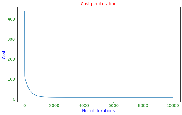
print ('Minimized cost:', loss(b, m, data))
Optimized b: 37.27234604666433
Optimized m: -5.340801130745784
Minimized cost: 8.697573986717137
fig, ax = plt.subplots(figsize=(10,6))
plt.plot(cost_graph)
ax.set_xlabel('No. of iterations',fontsize=14,color='blue')
ax.set_ylabel('Cost',fontsize=14,color='blue')
plt.title('Cost per iteration',color='red',fontsize=14)
plt.xticks(fontsize=14)
plt.yticks(fontsize=14)
ax.tick_params(axis='x', colors='forestgreen')
ax.tick_params(axis='y', colors='forestgreen')
plt.show()
from sklearn.linear_model import LinearRegression
# what is the shape of x?
x.shape
(32,)
model = LinearRegression()
model.fit(x.reshape(-1,1),y)
LinearRegression()In a Jupyter environment, please rerun this cell to show the HTML representation or trust the notebook.
On GitHub, the HTML representation is unable to render, please try loading this page with nbviewer.org.
LinearRegression()
model.coef_ , model.intercept_ # this is what the has learned
(array([-5.34447157]), 37.28512616734204)
x_range = np.linspace(np.min(x)-1,np.max(x)+1,2)
yhat = model.predict(x_range.reshape(-1,1))
#Plot dataset
plt.scatter(x, y,ec='k',color='cyan',alpha=0.6)
#Predict y values
pred = model.coef_ * x_range + model.intercept_
#Plot predictions as line of best fit
plt.plot(x_range, pred, c='g')
plt.xlim(0, 6)
plt.ylim(0, 50)
plt.xlabel('Independent Variable $X$',fontsize=14,color='navy')
plt.ylabel('Dependent Variable $Y$',fontsize=14,color='navy')
plt.grid(which='major', color ='grey', linestyle='-', alpha=0.8)
plt.grid(which='minor', color ='grey', linestyle='--', alpha=0.2)
plt.axvline(x=xb, color='red',linestyle='dashed')
plt.axhline(y=yb, color='purple',linestyle='dashed')
plt.tick_params(axis='x', color='navy')
plt.tick_params(axis='y', color='navy')
plt.minorticks_on()
plt.title('Line of best fit',fontsize=14)
plt.legend(['Data','Trend','Mean of $X$','Mean of $Y$'])
plt.savefig('lineacorrelation.png',dpi=300)
plt.show()
model.score(x.reshape(-1,1),y)
0.7528327936582646
r**2
0.7528327936582647
###Test the Residuals for Goodness of fit
We investigate the distribution of the residuals, plot a histogram and apply a normality test
residuals = y - model.predict(x.reshape(-1,1))
import seaborn as sns

# import uniform distribution
from scipy import stats
from scipy.stats import norm
ax1 = sns.distplot(residuals,

                  bins=8,
                  kde=False,
                  color='deepskyblue',
                  hist_kws={"color":'green','ec':'black'},
                  fit=stats.norm,
                  fit_kws={"color":'red'})
ax1.set(xlabel='Residuals', ylabel='Frequency')
plt.show()
/usr/local/lib/python3.7/dist-packages/seaborn/distributions.py:2619: FutureWarning: `distplot` is a deprecated function and will be removed in a future version. Please adapt your code to use either `displot` (a figure-level function with similar flexibility) or `histplot` (an axes-level function for histograms).
  warnings.warn(msg, FutureWarning)
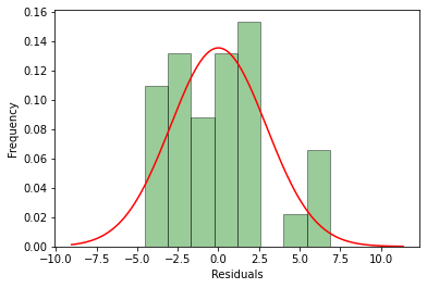
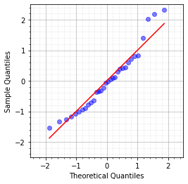
Message: The histogram does not quite look like a normal distribution. We can also consider a Q-Q Plot:#
import statsmodels.api as sm
sm.qqplot(residuals/np.std(residuals), loc = 0, scale = 1, line='s',alpha=0.5)
plt.xlim([-2.5,2.5])
plt.ylim([-2.5,2.5])
plt.axes().set_aspect('equal')
plt.grid(b=True,which='major', color ='grey', linestyle='-', alpha=0.5)
plt.grid(b=True,which='minor', color ='grey', linestyle='--', alpha=0.15)
plt.minorticks_on()
plt.show()
/usr/local/lib/python3.7/dist-packages/ipykernel_launcher.py:5: MatplotlibDeprecationWarning: Adding an axes using the same arguments as a previous axes currently reuses the earlier instance.  In a future version, a new instance will always be created and returned.  Meanwhile, this warning can be suppressed, and the future behavior ensured, by passing a unique label to each axes instance.
  """
dist = getattr(stats, 'norm')
params = dist.fit(residuals)
params
(-8.215650382226158e-15, 2.949162685955028)
# here we apply the test
stats.kstest(residuals, "norm", params)
KstestResult(statistic=0.08217402470387336, pvalue=0.9821261392158506)
The conclusion, in our case, is that the normality assumption is not violated.#
# for your convenience, this is the table with the critical values for the
# Kolmogorov-Smirnov test

def ks_critical_value(n_trials, alpha):
    return ksone.ppf(1-alpha/2, n_trials)

trials = range(1, 40)
alphas = [0.1, 0.05, 0.02, 0.01]

# Print table headers
print('{:<6}|{:<6} Level of significance, alpha'.format(' ', ' '))
print('{:<6}|{:>8} {:>8} {:>8} {:>8}'.format(*['Trials'] + alphas))
print('-' * 42)
# Print critical values for each n_trials x alpha combination
for t in trials:
    print('{:6d}|{:>8.5f} {:>8.5f} {:>8.5f} {:>8.5f}'
          .format(*[t] + [ks_critical_value(t, a) for a in alphas]))
    if t % 10 == 0:
        print()
ks_critical_value(31,0.4)
0.15594527177147208
A different normality test indicates the same thing#
stats.anderson(residuals,dist='norm')
AndersonResult(statistic=0.46842144463906266, critical_values=array([0.523, 0.596, 0.715, 0.834, 0.992]), significance_level=array([15. , 10. , 5. , 2.5, 1. ]))
stats.shapiro(residuals)
(0.9450768828392029, 0.10438867658376694)
#@title
model = sm.OLS(y, x)
results = model.fit()
print(results.summary())
x = cars.iloc[:,2:8]
x
| cyl | disp | hp | drat | wt | qsec | |
|---|---|---|---|---|---|---|
| 0 | 6 | 160.0 | 110 | 3.90 | 2.620 | 16.46 |
| 1 | 6 | 160.0 | 110 | 3.90 | 2.875 | 17.02 |
| 2 | 4 | 108.0 | 93 | 3.85 | 2.320 | 18.61 |
| 3 | 6 | 258.0 | 110 | 3.08 | 3.215 | 19.44 |
| 4 | 8 | 360.0 | 175 | 3.15 | 3.440 | 17.02 |
| 5 | 6 | 225.0 | 105 | 2.76 | 3.460 | 20.22 |
| 6 | 8 | 360.0 | 245 | 3.21 | 3.570 | 15.84 |
| 7 | 4 | 146.7 | 62 | 3.69 | 3.190 | 20.00 |
| 8 | 4 | 140.8 | 95 | 3.92 | 3.150 | 22.90 |
| 9 | 6 | 167.6 | 123 | 3.92 | 3.440 | 18.30 |
| 10 | 6 | 167.6 | 123 | 3.92 | 3.440 | 18.90 |
| 11 | 8 | 275.8 | 180 | 3.07 | 4.070 | 17.40 |
| 12 | 8 | 275.8 | 180 | 3.07 | 3.730 | 17.60 |
| 13 | 8 | 275.8 | 180 | 3.07 | 3.780 | 18.00 |
| 14 | 8 | 472.0 | 205 | 2.93 | 5.250 | 17.98 |
| 15 | 8 | 460.0 | 215 | 3.00 | 5.424 | 17.82 |
| 16 | 8 | 440.0 | 230 | 3.23 | 5.345 | 17.42 |
| 17 | 4 | 78.7 | 66 | 4.08 | 2.200 | 19.47 |
| 18 | 4 | 75.7 | 52 | 4.93 | 1.615 | 18.52 |
| 19 | 4 | 71.1 | 65 | 4.22 | 1.835 | 19.90 |
| 20 | 4 | 120.1 | 97 | 3.70 | 2.465 | 20.01 |
| 21 | 8 | 318.0 | 150 | 2.76 | 3.520 | 16.87 |
| 22 | 8 | 304.0 | 150 | 3.15 | 3.435 | 17.30 |
| 23 | 8 | 350.0 | 245 | 3.73 | 3.840 | 15.41 |
| 24 | 8 | 400.0 | 175 | 3.08 | 3.845 | 17.05 |
| 25 | 4 | 79.0 | 66 | 4.08 | 1.935 | 18.90 |
| 26 | 4 | 120.3 | 91 | 4.43 | 2.140 | 16.70 |
| 27 | 4 | 95.1 | 113 | 3.77 | 1.513 | 16.90 |
| 28 | 8 | 351.0 | 264 | 4.22 | 3.170 | 14.50 |
| 29 | 6 | 145.0 | 175 | 3.62 | 2.770 | 15.50 |
| 30 | 8 | 301.0 | 335 | 3.54 | 3.570 | 14.60 |
| 31 | 4 | 121.0 | 109 | 4.11 | 2.780 | 18.60 |
model.fit(x,y)
LinearRegression(copy_X=True, fit_intercept=True, n_jobs=None, normalize=False)
model.score(x,y)
0.8548224115848234
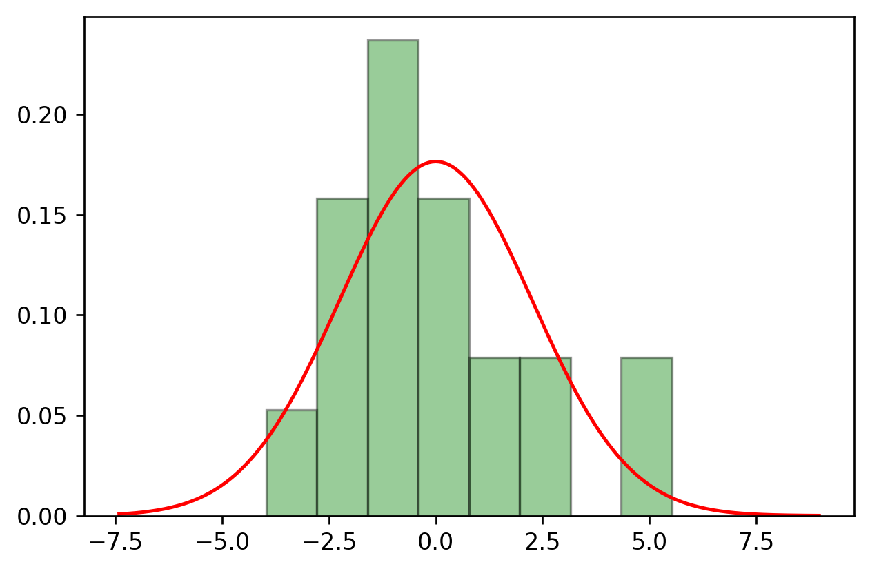
residuals = y - model.predict(x)
sns.distplot(residuals,
                  bins=8,
                  kde=False,
                  color='deepskyblue',
                  hist_kws={"color":'green','ec':'black'},
                  fit=stats.norm,
                  fit_kws={"color":'red'})
plt.show()
/usr/local/lib/python3.7/dist-packages/seaborn/distributions.py:2619: FutureWarning: `distplot` is a deprecated function and will be removed in a future version. Please adapt your code to use either `displot` (a figure-level function with similar flexibility) or `histplot` (an axes-level function for histograms).
  warnings.warn(msg, FutureWarning)
dist = getattr(stats, 'norm')
params = dist.fit(residuals)
# here we apply the Kolmogorov-Smirnov test
stats.kstest(residuals, "norm", params) # the confidence has increased compared to the case of using only one input feature.
KstestResult(statistic=0.15722261669146254, pvalue=0.37091468826166857)