Dimensionality Reduction and Unsupervised Learning (K-Means)#
Principal Component Analysis (PCA) #
Case Study 1:
Suppose we have only one input variable whose value is constant and a continuous target variable that has a significant coefficient of variation.
Can this data alone be used for making a predictive model with a high R-2 score?
Case Study 2:
Suppose we have only one input feature in the data that has a lot of variability, but the linear correlation coefficient with the designated target variable is 0.
What can we infer from this situation? Would any model of regression fail?
Case Study 3:
Suppose we have only one input feature in the data that has a lot of variability, but the linear correlation coefficient with the designated target variable is 0.
What can we infer from this situation? Would any model of regression fail?
Principal Components in 2-D #
 |
 |
Finding the first principal component is equivalent to finding the coefficients that maximize the variance of the linear combination:
Exercise: Given data with two features find the linear combination whose variance is maximum.
Important: how is the second principal component constructed?
Important: would it be a good idea to scale the variables before computing the principal components?
Formal Math #
Center the data: Subtract the mean of \(F_1\) from each \(F_1\) value, and subtract the mean of \(F_2\) from each \(F_2\) value. This ensures your data is centered around the origin.
Compute the covariance matrix: Calculate the 2x2 covariance matrix:
\begin{align} \begin{bmatrix} \operatorname{Cov}(F1, F1) & \operatorname{Cov}(F1, F2)\ \operatorname{Cov}(F2, F1) & \operatorname{Cov}(F2, F2) \end{bmatrix} \end{align}
Compute the Eigenvalues/Eigenvectors: Find the eigenvectors and eigenvalues of the covariance matrix. The eigenvector corresponding to the largest eigenvalue is the direction of the first principal component.
Representation: This eigenvector represents the coefficients for the first principal component. Let’s say the first eigenvector is \((\beta_1,\beta_2)\). Then the first principal component (PC1) is calculated as: $\(\beta_1\cdot F_1 + \beta_2\cdot F_2.\)$
Representing Variability#
 |
 |
A stripplot shows a visualization for the amount of variability in the orginal feature values compared to the principal components.
PCA in Multiple Dimensions #
Message: PCA creates new variables that are linear combinations of the original variables, and capture decreasing amounts of variability from the data.

 |
 |
Patterns #
PCA does not cluster data, but we can still look for patterns; methods such as KMeans++ could help further.
 |
 |
t-Stochastic Neighbor Embeddings (tSNE) #
Why another Dimensionality Reduction method?#
PCA aims at preserving the global structure; however it focuses on finding directions (principal components) that maximize the variance explained in the data.
PCA is a linear method. Finds linear combinations of features that best explain the variance.
The principal components are orthogonal vectors.
Principal components can often be interpreted for their meaning, and the distances between points on the plot may hold more importance. Think of principal components as a change of coordinates for a space (formally, this is a vector subspace spanned by the features.)
Critical Thinking: can we imagine a data set whose important aspects may not be captured efficiently by the principal components?
Examples: Is there a direction along which we can maximize the variability and help solve the classification problems below?
 |
 |
A manifold learning method is proposed: t-SNE (L. van der Maaten, G. Hinton - 2008) #
References:
https://www.jmlr.org/papers/volume9/vandermaaten08a/vandermaaten08a.pdf
https://torontolife.com/tech/ai-superstars-google-facebook-apple-studied-guy/
Purpose:
t-SNE: Designed specifically for visualization of high-dimensional data. It excels at creating visual representations that emphasize local clusters and relationships.
PCA: Primarily a dimensionality reduction technique for general purposes. It focuses on finding directions (principal components) that maximize the variance explained in the data.
Linearity:
t-SNE: Nonlinear method. It can capture complex, curved structures in the data.
PCA: Linear method. Finds linear combinations of features that best explain the variance.
Aims:
t-SNE: Preserves local similarity. Points that are close in the high-dimensional space tend to be clustered together in the low-dimensional representation.
PCA: Preserves global structure. It focuses on maximizing the variance explained across the entire dataset.
Main Ideas and Concepts #
t-SNE is a form of non-linear dimensionality reduction (manifold learning.)
Important: it matters how you compute distances, and also how the algorithm perceives local structures.
Geodesic distance: the shortest curve on a manifold that connects two points.
 |
 |
Image source: https://www.cs.cmu.edu/~bapoczos/Classes/ML10715_2015Fall/slides/ManifoldLearning.pdf
How t-SNE works #
“Stochastic Neighbor Embedding (SNE) starts by converting the high-dimensional Euclidean distances between datapoints into conditional probabilities that represent similarities. The similarity of datapoint \( x_j\) to datapoint \(x_i\) is the conditional probability, \(p_{j|i}\), that \( x_i\) would pick \( x_j \) as its neighbor if neighbors were picked in proportion to their probability density under a Gaussian centered at \( x_i \). For nearby datapoints, \( p_{j|i} \) is relatively high, whereas for widely separated datapoints, \( p_{j|i} \) will be almost infinitesimal (for reasonable values of the variance of the Gaussian, \( \sigma_i \)). Mathematically, the conditional probability \(p_{j|i}\) is given by
where \( p_{j|i} \) is the probability that point \(x_i\) picks point \(x_j\) as its neighbor.”
From a multidimensional space we get similarity scores.
 |
|

The method has defined a cost function that will be minimized iteratively to obtain an optimal embedding given a perplexity value that indirectly controls the widths (variances) of the Gaussian distributions. A higher perplexity value leads to wider Gaussian distributions, considering a broader neighborhood of points. The cost function \(C\) is given by
Low Dimensional Space Embeddings #
t-Distribution: In the low-dimensional space, t-SNE doesn’t use Gaussians. It uses a heavier-tailed t-distribution to better model the embedding.
Optimization: t-SNE works by trying to make the probability distributions in the high and low-dimensional spaces as similar as possible.
Key point: While t-SNE conceptually uses multivariate Gaussian distributions to represent neighborhood structure in the original high-dimensional data, the visualization process involves nonlinear transformations and a shift to using t-distributions.
Perplexity #
Perplexity: is a measure of local neighborhood Size. Think of perplexity as a target number of “effective neighbors” for each data point. A higher perplexity signifies considering a broader neighborhood, while a lower perplexity focuses on a tighter cluster of close neighbors.
Impact on Gaussian Distributions (Conceptual): Imagine a Gaussian distribution centered on each data point in the high-dimensional space. t-SNE uses these Gaussians to capture the similarity between neighboring points. The perplexity value influences the variance of these Gaussians. Higher perplexity leads to wider Gaussians, encompassing a larger neighborhood and capturing broader relationships. Lower perplexity results in narrower Gaussians, focusing on more immediate, highly similar neighbors.
Choosing the Right Perplexity: Unfortunately, there’s no single “best” perplexity value for all datasets.
Here are some common strategies for selecting perplexity:
Experiment with a range of values and visually compare the resulting t-SNE plots. Look for a balance between capturing clusters and preserving some global structure.
Think about the intrinsic dimensionality of your data. Lower perplexity might be suitable for data with already well-defined clusters.
Consider perplexity values between 5 and 50 as a starting point for exploration.
While perplexity is a critical parameter, it’s not the only factor affecting t-SNE results. Learning rate and the number of iterations can also influence the outcome.
Perplexity doesn’t directly map to a specific number of neighbors. It’s a smoother measure of effective neighbors, accounting for the distribution of similarities.
Unsupervised Learning - KMeans Algorithm #
Introduction#
KMeans is one of the most widely used clustering algorithms in machine learning and data mining. It is an unsupervised learning algorithm that aims to partition a dataset into K distinct, non-overlapping subsets (clusters) based on feature similarity. Each data point belongs to the cluster with the nearest mean, serving as a prototype of the cluster.
Key Concepts #
Clusters: Groupings of data points such that points in the same group are more similar to each other than to those in other groups.
Centroids: The center of a cluster. In KMeans, each cluster is represented by its centroid, which is the mean of all points in the cluster.
Steps of the KMeans Algorithm #
Initialization: Select K initial centroids randomly from the data points.
Assignment: Assign each data point to the nearest centroid based on the Euclidean distance.
Update: Calculate new centroids by taking the mean of all data points assigned to each cluster.
Repeat: Repeat the assignment and update steps until the centroids no longer change significantly or a maximum number of iterations is reached.
Details #
Initialization:
Choose K initial centroids randomly from the dataset.
These centroids will serve as the starting points for the clusters.
Assignment:
For each data point, calculate the Euclidean distance to each centroid.
Assign the data point to the cluster with the nearest centroid.
This step creates K clusters with assigned data points.
Update:
Recalculate the centroid of each cluster as the mean of all data points assigned to that cluster.
The new centroid is the arithmetic mean of the points in the cluster.
Repeat:
Repeat the assignment and update steps until convergence is achieved (i.e., centroids do not change significantly between iterations) or a predetermined number of iterations is reached.
Convergence #
The KMeans algorithm aims to minimize the within-cluster sum of squares (WCSS), also known as inertia. WCSS measures the compactness of the clusters and is defined as the sum of the squared distances between each data point and its corresponding centroid. The goal is to achieve clusters where the data points are as close as possible to their respective centroids.
Advantages #
Simplicity: KMeans is easy to understand and implement.
Scalability: It is efficient for large datasets.
Speed: The algorithm converges quickly.
Disadvantages #
Initialization Sensitivity: The quality of the final clusters depends heavily on the initial choice of centroids. Poor initialization can lead to suboptimal clustering.
Fixed Number of Clusters: The user must specify the number of clusters (K) beforehand, which might not be known.
Spherical Clusters: KMeans assumes that clusters are spherical and of similar size, which may not be the case for all datasets.
Outliers Sensitivity: KMeans is sensitive to outliers, which can distort the clustering results.
Takeaways #
KMeans is a foundational clustering algorithm that partitions data into K clusters based on feature similarity. Despite its simplicity and efficiency, it has limitations related to initialization sensitivity, the requirement to specify the number of clusters, and assumptions about cluster shape and size. Enhancements like KMeans++ have been developed to address some of these issues, improving the initialization process and overall clustering performance.
Understanding KMeans is essential for anyone working with clustering and unsupervised learning, as it provides a basis for more advanced clustering techniques and insights into the structure of complex datasets.
An Upgrade: KMeans++ #
KMeans++ is an initialization algorithm for the KMeans clustering method, designed to improve the convergence speed and quality of the final clustering results. KMeans clustering is a popular unsupervised learning algorithm used to partition a dataset into K distinct clusters based on feature similarity. The traditional KMeans algorithm has a major drawback: its performance and the quality of the resulting clusters heavily depend on the initial placement of the centroids. Poor initialization can lead to suboptimal clustering and slow convergence. KMeans++ addresses this issue by providing a smarter way to initialize the centroids.
Traditional KMeans Algorithm #
Before exploring the upgrades implemented by KMeans++, it’s essential to understand the traditional KMeans algorithm:
Initialization: Randomly select K data points as initial centroids.
Assignment: Assign each data point to the nearest centroid, forming K clusters.
Update: Calculate the new centroids as the mean of the data points assigned to each cluster.
Repeat: Repeat the assignment and update steps until the centroids no longer change significantly or a maximum number of iterations is reached.
Limitations of Traditional KMeans #
The primary limitation of the traditional KMeans algorithm is its sensitivity to the initial centroid positions. Poor initialization can result in:
Slow convergence: More iterations are needed to reach the final clustering.
Poor clustering quality: Suboptimal clusters with high within-cluster variance.
KMeans++ Initialization #
KMeans++ improves the initial selection of centroids, leading to better clustering performance. The steps of the KMeans++ initialization are as follows:
Randomly select the first centroid from the data points.
For each subsequent centroid:
Compute the distance (squared Euclidean distance) between each data point and the nearest centroid that has already been chosen.
Select the next centroid from the data points with a probability proportional to the squared distance (data points farther from the existing centroids have a higher chance of being selected).
Repeat step 2 until K centroids are chosen.
Advantages of KMeans++ #
Improved Convergence: By starting with well-spread centroids, KMeans++ typically converges faster than traditional KMeans.
Better Clustering Quality: The initial centroids are more likely to be close to the final cluster centers, leading to lower within-cluster variance and more accurate clustering.
Reduced Sensitivity to Initial Centroids: KMeans++ reduces the impact of poor initial centroid selection, making the algorithm more robust.
Main Takeaways #
KMeans++ is a significant improvement over the traditional KMeans algorithm, providing better initialization of centroids, which leads to faster convergence and higher-quality clustering results. It is widely used in practice and is the default initialization method in many KMeans implementations, including those in popular machine learning libraries like scikit-learn.
By reducing the dependency on initial centroid positions, KMeans++ makes the KMeans clustering algorithm more robust and effective, especially for large and complex datasets.
Code Applications #
Setup#
import os
if 'google.colab' in str(get_ipython()):
  print('Running on CoLab')
  !pip install -q hdbscan
  from google.colab import drive
  drive.mount('/content/drive')
  os.chdir('/content/drive/My Drive/Data Sets')
else:
  print('Running locally')
  os.chdir('../Data')
Running on CoLab
     ━━━━━━━━━━━━━━━━━━━━━━━━━━━━━━━━━━━━━━━━ 3.6/3.6 MB 9.7 MB/s eta 0:00:00
     ━━━━━━━━━━━━━━━━━━━━━━━━━━━━━━━━━━━━━━━━ 1.9/1.9 MB 19.2 MB/s eta 0:00:00
?25hDrive already mounted at /content/drive; to attempt to forcibly remount, call drive.mount("/content/drive", force_remount=True).
# Library Setup
import numpy as np
import hdbscan
%matplotlib inline
%config InlineBackend.figure_format = 'retina'
import matplotlib.pyplot as plt
import plotly.graph_objs as go
import plotly.express as px
import seaborn as sns
from matplotlib import style
style.use("ggplot")
from sklearn.cluster import KMeans
from sklearn.decomposition import PCA
from sklearn.manifold import TSNE
from sklearn.datasets import load_wine
import matplotlib.pyplot as plt
from mpl_toolkits.mplot3d import Axes3D
from sklearn.datasets import make_swiss_roll
from sklearn.preprocessing import StandardScaler
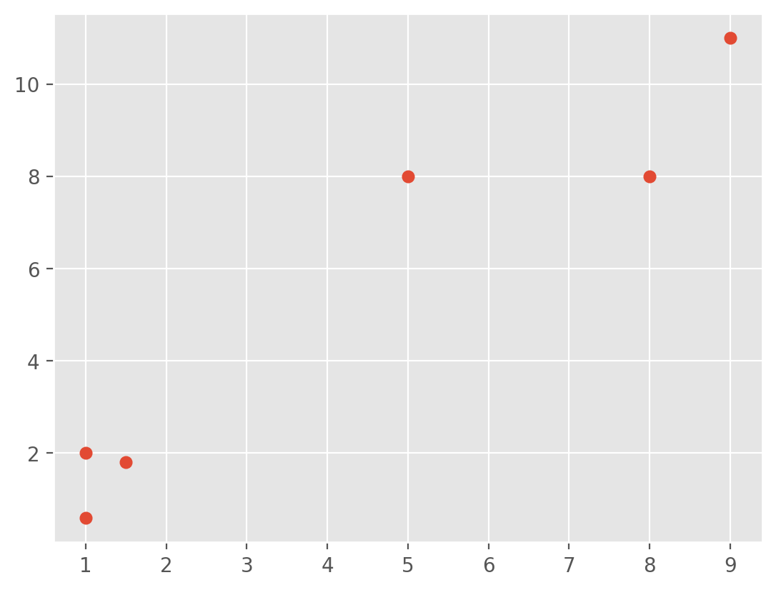
KMeans Example#
x = [1, 5, 1.5, 8, 1, 9]
y = [2, 8, 1.8, 8, 0.6, 11]
plt.scatter(x,y)
plt.show()
X = np.array([[1, 2],
[5, 8],
[1.5, 1.8],
[8, 8],
[1, 0.6],
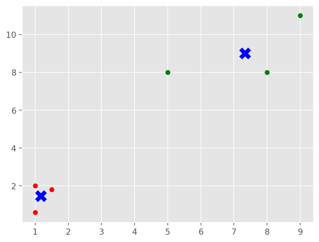
[9, 11]])
kmeans = KMeans(n_clusters=2,n_init='auto')
kmeans.fit(X)
centroids = kmeans.cluster_centers_
labels = kmeans.labels_
print(centroids)
print(labels)
colors = ["g.","r.","c.","y."]
for i in range(len(X)):
print("coordinate:",X[i], "label:", labels[i])
plt.plot(X[i][0], X[i][1], colors[labels[i]], markersize = 10)
plt.scatter(centroids[:, 0],centroids[:, 1], marker = "x", s=120,color='blue', linewidths = 5, zorder = 10)
plt.show()
[[7.33333333 9.        ]
 [1.16666667 1.46666667]]
[1 0 1 0 1 0]
coordinate: [1. 2.] label: 1
coordinate: [5. 8.] label: 0
coordinate: [1.5 1.8] label: 1
coordinate: [8. 8.] label: 0
coordinate: [1.  0.6] label: 1
coordinate: [ 9. 11.] label: 0
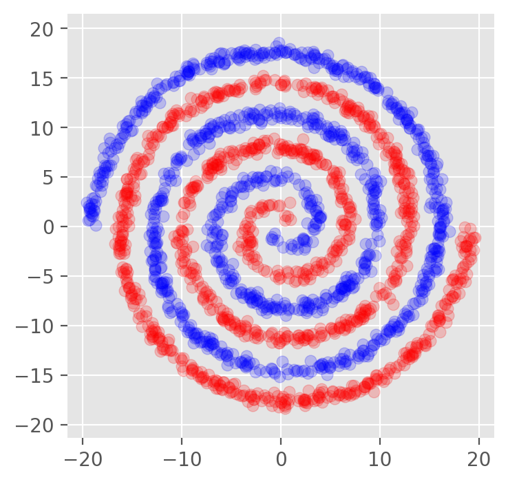
Dimensionality Reduction Applications#
N = 1000  # The number of points per arm
S = 0.1   # The distance of the first points from the center of the spiral
L = 6.0   # The length of the spiral in number of turns
W = 0.35  # The thickness of the spirals arms

theta = np.sqrt(np.random.rand(N)) * L * np.pi

r_a = theta + np.pi * S
data_a = np.array([np.cos(theta) * r_a, np.sin(theta) * r_a]).T
x_a = data_a + np.random.randn(N, 2) * W

r_b = -1 * theta - np.pi * S
data_b = np.array([np.cos(theta) * r_b, np.sin(theta) * r_b]).T
x_b = data_b + np.random.randn(N, 2) * W

res_a = np.append(x_a, np.zeros((N,1)), axis=1)
res_b = np.append(x_b, np.ones((N,1)), axis=1)
res = np.append(res_a, res_b, axis=0)

np.random.shuffle(res)

np.savetxt("spiral.csv", res, delimiter=",", header="x,y,label", comments="", fmt='%.5f')

fig, ax = plt.subplots(figsize=(4,4))
ax.spines['top'].set_visible(False)
ax.spines['right'].set_visible(False)
ax.spines['bottom'].set_visible(False)
ax.spines['left'].set_visible(False)
ax.set_xlim(-20, 20)
ax.set_ylim(-20, 20)
# ax.grid(which='major', color ='grey', linestyle='-', alpha=0.8)
# ax.grid(which='minor', color ='grey', linestyle='--', alpha=0.2)
# ax.minorticks_on()
plt.scatter(x_a[:,0],x_a[:,1],color='r',alpha=0.2)
plt.scatter(x_b[:,0],x_b[:,1],color='b',alpha=0.2)
plt.axis('equal')
plt.savefig('spiral.png',dpi=300)
plt.show()
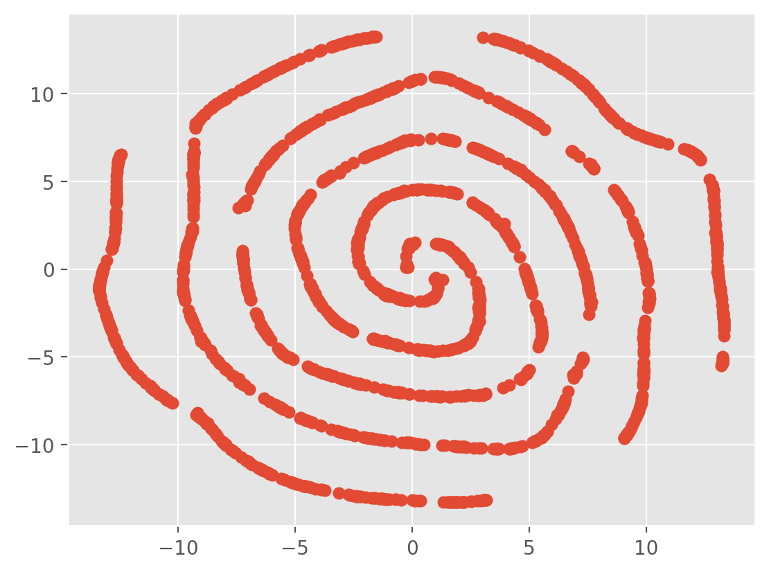
data = np.row_stack((x_a, x_b))
tsne = TSNE(n_components=2, verbose=1, perplexity=20, n_iter=300)
tsne_results = tsne.fit_transform(data)
[t-SNE] Computing 61 nearest neighbors...
[t-SNE] Indexed 2000 samples in 0.002s...
[t-SNE] Computed neighbors for 2000 samples in 0.034s...
[t-SNE] Computed conditional probabilities for sample 1000 / 2000
[t-SNE] Computed conditional probabilities for sample 2000 / 2000
[t-SNE] Mean sigma: 1.176694
[t-SNE] KL divergence after 250 iterations with early exaggeration: 54.913757
[t-SNE] KL divergence after 300 iterations: 1.135829
plt.scatter(tsne_results[:,0], tsne_results[:,1])
plt.show()
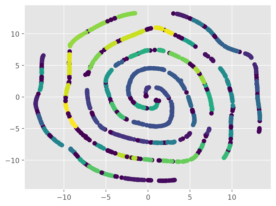
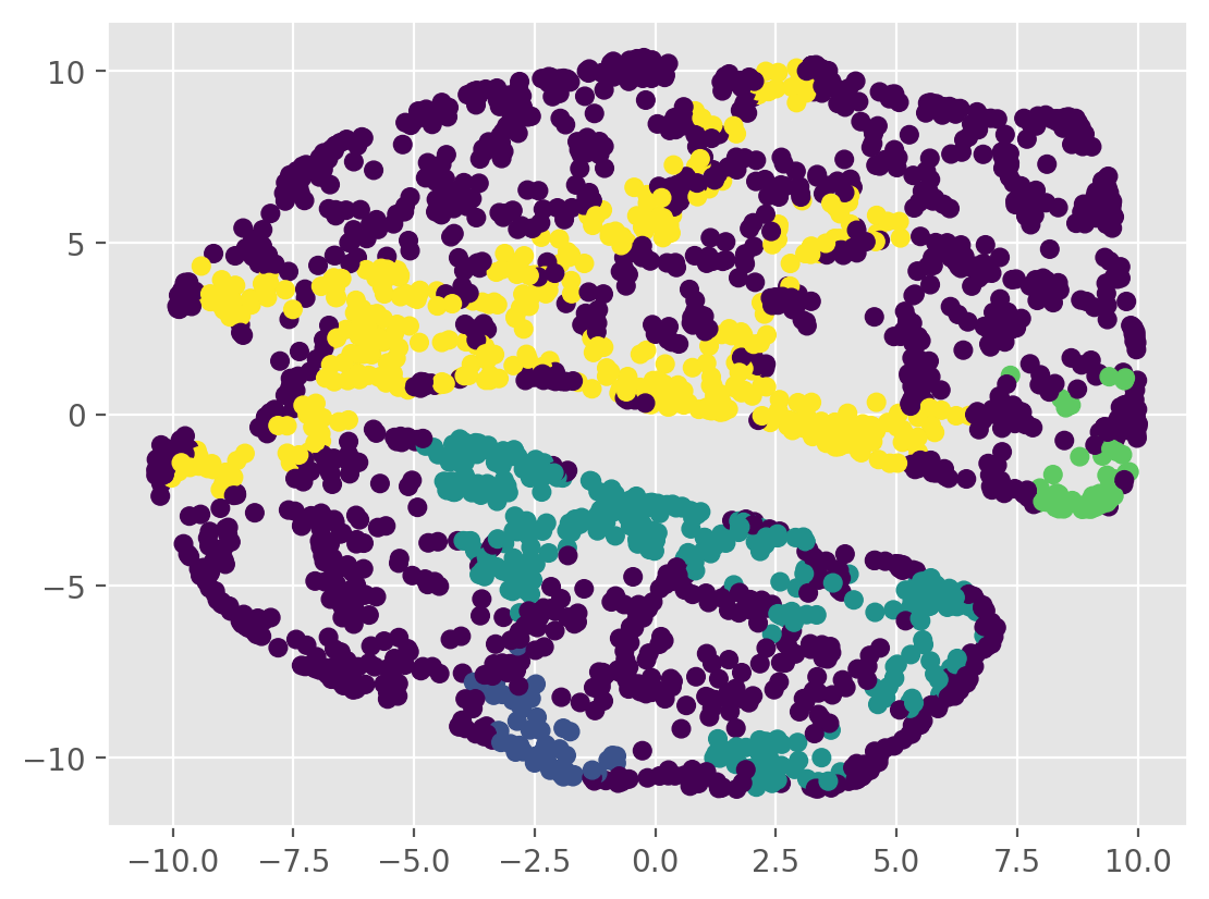
# clusetering with HDBScan
hdbscan_model = hdbscan.HDBSCAN(min_cluster_size=10)
labels = hdbscan_model.fit_predict(tsne_results)

# Plot the clusters
plt.scatter(tsne_results[:, 0], tsne_results[:, 1], c=labels)
plt.show()
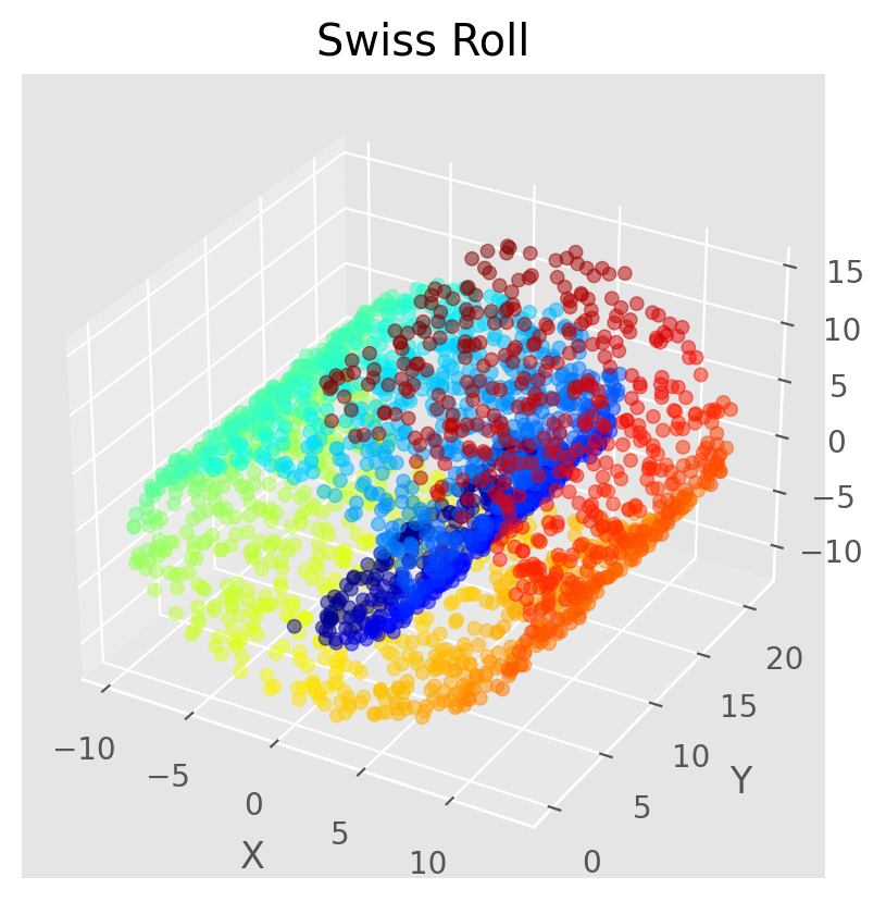
# Generate the Swiss roll dataset
X, t = make_swiss_roll(n_samples=2500, noise=0.2, random_state=123)

# Create a 3D plot
fig = plt.figure()
ax = fig.add_subplot(111, projection='3d')

# Scatter plot with color gradient based on t
ax.scatter(X[:, 0], X[:, 1], X[:, 2], c=t, cmap='jet', s=20,alpha=0.5)

# Add labels and title
ax.set_xlabel('X')
ax.set_ylabel('Y')
ax.set_zlabel('Z')
ax.set_title('Swiss Roll')

plt.show()
# Create a DataFrame for easy handling in Plotly
import pandas as pd
df = pd.DataFrame({'x': X[:, 0], 'y': X[:, 1], 'z': X[:, 2], 'color': t})

# Generate 3D scatter plot with Plotly
fig = px.scatter_3d(df, x='x', y='y', z='z', color='color')

# Customize appearance (optional)
fig.update_layout(margin=dict(l=0, r=0, b=0, t=0))

fig.show()
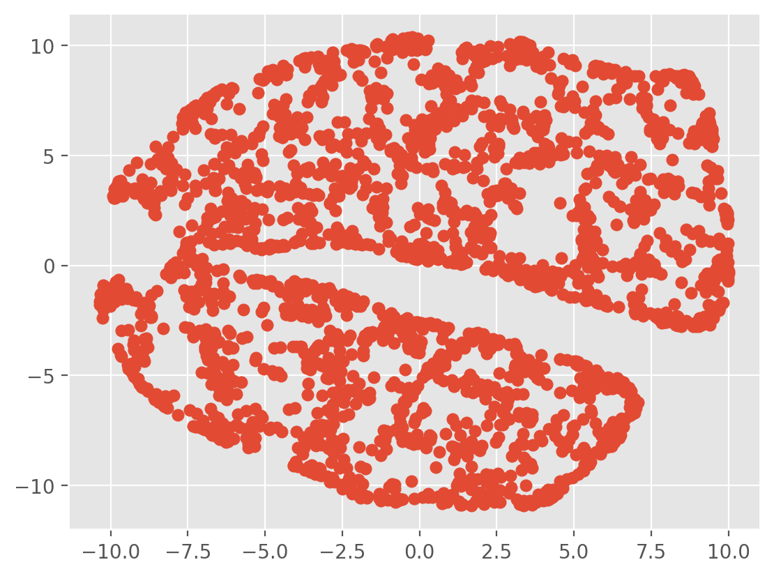
tsne = TSNE(n_components=2, verbose=1, perplexity=40, n_iter=300)
tsne_results = tsne.fit_transform(X)
[t-SNE] Computing 121 nearest neighbors...
[t-SNE] Indexed 2500 samples in 0.008s...
[t-SNE] Computed neighbors for 2500 samples in 0.134s...
[t-SNE] Computed conditional probabilities for sample 1000 / 2500
[t-SNE] Computed conditional probabilities for sample 2000 / 2500
[t-SNE] Computed conditional probabilities for sample 2500 / 2500
[t-SNE] Mean sigma: 1.866024
[t-SNE] KL divergence after 250 iterations with early exaggeration: 59.205956
[t-SNE] KL divergence after 300 iterations: 1.203116
plt.scatter(tsne_results[:,0], tsne_results[:,1])
plt.show()
# Fit HDBSCAN model
hdbscan_model = hdbscan.HDBSCAN(min_cluster_size=50)
labels = hdbscan_model.fit_predict(tsne_results)

# Plot the clusters
plt.scatter(tsne_results[:, 0], tsne_results[:, 1], c=labels)
plt.show()
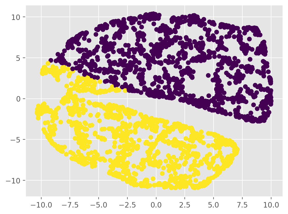
kmeans = KMeans(n_clusters=2,n_init='auto')
kmeans.fit(tsne_results)
centroids = kmeans.cluster_centers_
labels = kmeans.labels_
print(centroids)
print(labels)
[[ 2.19155    4.2587166]
 [-2.310304  -4.6294637]]
[1 0 0 ... 1 0 1]
# Plot the clusters
plt.scatter(tsne_results[:, 0], tsne_results[:, 1], c=labels)
plt.show()
Data Application#
wine = load_wine()
X = wine.data
X_names = wine.feature_names
y = wine.target
scale = StandardScaler()
Xs = scale.fit_transform(X)
pd.DataFrame(Xs, columns=X_names).head()
| alcohol | malic_acid | ash | alcalinity_of_ash | magnesium | total_phenols | flavanoids | nonflavanoid_phenols | proanthocyanins | color_intensity | hue | od280/od315_of_diluted_wines | proline | |
|---|---|---|---|---|---|---|---|---|---|---|---|---|---|
| 0 | 1.518613 | -0.562250 | 0.232053 | -1.169593 | 1.913905 | 0.808997 | 1.034819 | -0.659563 | 1.224884 | 0.251717 | 0.362177 | 1.847920 | 1.013009 |
| 1 | 0.246290 | -0.499413 | -0.827996 | -2.490847 | 0.018145 | 0.568648 | 0.733629 | -0.820719 | -0.544721 | -0.293321 | 0.406051 | 1.113449 | 0.965242 |
| 2 | 0.196879 | 0.021231 | 1.109334 | -0.268738 | 0.088358 | 0.808997 | 1.215533 | -0.498407 | 2.135968 | 0.269020 | 0.318304 | 0.788587 | 1.395148 |
| 3 | 1.691550 | -0.346811 | 0.487926 | -0.809251 | 0.930918 | 2.491446 | 1.466525 | -0.981875 | 1.032155 | 1.186068 | -0.427544 | 1.184071 | 2.334574 |
| 4 | 0.295700 | 0.227694 | 1.840403 | 0.451946 | 1.281985 | 0.808997 | 0.663351 | 0.226796 | 0.401404 | -0.319276 | 0.362177 | 0.449601 | -0.037874 |
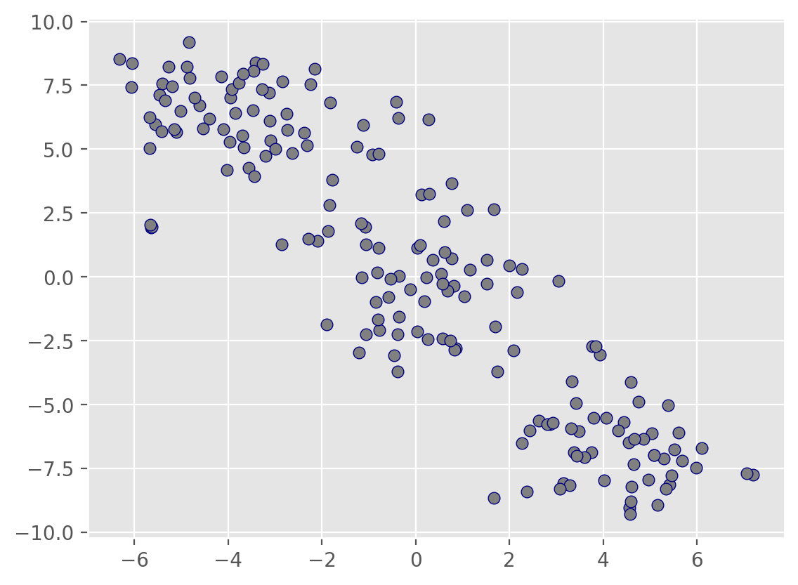
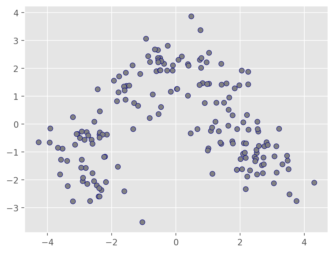
# dimensionality reduction with PCA
pca = PCA()
Xs_pca = pca.fit_transform(Xs)
plt.scatter(Xs_pca[:,0], Xs_pca[:,1],color="grey",ec='navy')
plt.show()
# clustering with hdbscan
hdbscan_model = hdbscan.HDBSCAN(min_cluster_size=17)
labels = hdbscan_model.fit_predict(Xs_pca)

# Plot the clusters
plt.scatter(Xs_pca[:, 0], Xs_pca[:, 1], c=labels)
plt.show()
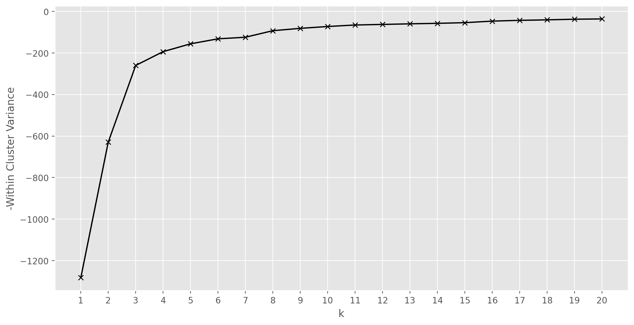
# clustering with KMeans, the optimal number of clusters based on minimization of intraclass variance
scores=[]
k_range = np.arange(1,21)
for k in k_range:
    km = KMeans(n_clusters=k, n_init='auto',random_state=123)
    km.fit(Xs_pca[:,:2])
    scores.append(km.score(Xs_pca[:,:2]))

plt.figure(figsize=(12,6))
plt.plot(k_range, scores, '-xk')
plt.xlabel('k')
plt.xticks(k_range)
plt.ylabel('-Within Cluster Variance')
plt.show()
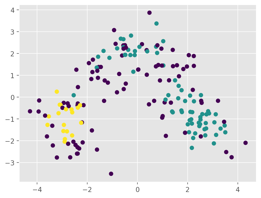
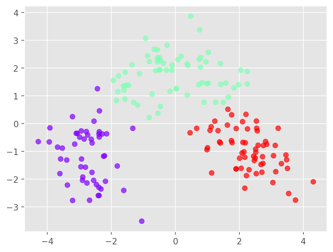
k = 3
km = KMeans(n_clusters=k, n_init='auto',random_state=146)
labels = km.fit_predict(Xs_pca[:,:2])
# Plot the clusters
plt.scatter(Xs_pca[:, 0], Xs_pca[:, 1], c=labels,cmap='rainbow',alpha=0.7)
plt.show()
# dimensionality reduction with tSNE
tsne = TSNE(n_components=2, verbose=1, perplexity=40, n_iter=300)
Xs_tsne = tsne.fit_transform(Xs)
[t-SNE] Computing 121 nearest neighbors...
[t-SNE] Indexed 178 samples in 0.001s...
[t-SNE] Computed neighbors for 178 samples in 0.006s...
[t-SNE] Computed conditional probabilities for sample 178 / 178
[t-SNE] Mean sigma: 1.839161
[t-SNE] KL divergence after 250 iterations with early exaggeration: 48.587795
[t-SNE] KL divergence after 300 iterations: 0.324551
plt.scatter(Xs_tsne[:,0], Xs_tsne[:,1],color="grey",ec='navy')
plt.show()