Introduction, Bias Variance Tradeoff and Gradient Descent

Data Science

• Data is information, a perception of our own existence and everything surrounding us.

• The amount of data that we can record nowadays exceeds anything accomplished before.

• 1 bit = 0 or 1.

• letter = 1 byte = 8 bits, such as for example \((0,1,1,0,0,1,1,0).\)

Critical Thinking: We need many “letters” to encode information! How many different “letters” do we have? Hint: Use the multiplication principle.

• 1000 letters = 1kbyte = \(10^3\) bytes.

• 1 mil. letters = 1 mbyte = \(10^3\) kbytes.

• 1 gbyte = 1 bil. letters = \(10^3\) mbytes.

• 1 tbyte = \(10^3\) gbytes, (tbyte means terabyte).

• 1 pbyte = \(10^3\) tbytes, (pbyte means petabyte).

• 1 ebyte = \(10^3\) pbytes, (ebyte means exabyte).

Machine Learning

Suggested References:

The Hundred-Page Book of Machine Learning

Probabilistic Machine Learning - An Introduction

Who said “machine-learning?”

https://www.ibm.com/cloud/learn/machine-learning

In a few words, it is the science of automating and improving decisions and inferences based on data.

Types of Data

• Data could be classified based on the levels of measurement, such as nominal, ordinal, interval and ratio.

• Nominal data: unique identifiers but order does not matter for example, peoples’ names, names of flowers, colors etc.

• Ordinal data: unique indentifiers and order matters, such as in letter grades, military or administration ranks, etc.

• Continuous data: Interval level of measurement: numerical values where differences make sense in the context of using them but ratios or proportions could be meaningless, such as temperatures, heights of people, days in the calendar.

• Continuous data: Ratio level of measurement: numerical values, that are at the interval level of measurement and also the ratio and proportions make sense in the context of using them, such as salaries, weights, distances, forces, etc.

Types of Data - Example

Independent vs Dependent variables:

Country	Age	Salary	Purchased
France	44	72000	No
Spain	29	51000	Yes
Germany	32	63000	No
Japan	53	81000	Yes
Portugal	48	73000	Yes
Italy	43	67500	No

In this example, the variables “Country”, “Age” and “Salary” are independent whereas “Purchased” is a dependent variable.

Quite often in the Data Science community nominal variables are referred as “discrete”.

CRITICAL THINKING: the context and the implied usage is very important for determining the level of measurement.

Levels of Measurement

Machine Learning

• Machine learning is the science of programming computers for using data with the goal of automating predictions and analyses.

• In all, it consists of input-output algorithms for supervised and/or unsupervised learning.

• We learn how to apply machine learing algorithms implemented in Python in order to analyze and make predictions by using real data sets.

• Pyhton is a very popular and friendly to use interpreted programming language that has currently emerged with prominence in the Data Science commumity.

Programming Language: Python

For using Python you can access http://colab.research.google.com via an internet browser such as Chrome.

It is a scripting language that uses libraries of functions which must to be imported before using the specific functions needed.

Example:

import numpy as np
a = np.sin(np.pi/3)

This means that \(a=\sin(\frac{\pi}{3})=\frac{\sqrt{3}}{2}\)

Functions

Functions are a building block in Machine Learning. Every solution to a data problem is articulated in terms of functions.

A function is a mapping, a rule of correspondence such that an input is assigned exacly one output.

Crtical Thinking: Functions and Set Theory represent the building blocks of modern mathematics.

Example of a Function by Arrow Diagram

The important elements of a function are

i. the domain of the function
ii. the range (co-domain) of the function
iii. the definition of the function.

Object Oriented Programming

Introduction to Classes in Python

In Python, a class is a blueprint for creating objects. Objects are instances of classes, and classes define the properties (attributes) and behaviors (methods) that the objects created from the class can have. Classes are a fundamental concept in object-oriented programming (OOP) and allow for the creation of complex data structures and models.

Key Concepts

1. Class: A blueprint for creating objects. It defines a set of attributes and methods that the created objects can have.

2. Object: An instance of a class. Each object can have unique values for the attributes defined in the class.

3. Attributes: Variables that belong to a class or an instance of a class. They represent the properties or state of an object.

4. Methods: Functions defined within a class that describe the behaviors of the objects created from the class.

5. Inheritance: A way to form new classes using classes that have already been defined. It allows for the creation of a class that is a modified version of an existing class.

6. Encapsulation: The practice of keeping the details of the implementation hidden, only exposing the necessary parts of the code.

7. Polymorphism: The ability to present the same interface for different underlying data types.

Creating a Class

To create a class in Python, use the class keyword followed by the class name and a colon. Inside the class, you can define attributes and methods.

class MyClass:
    # Class attribute
    class_attribute = "I am a class attribute"

    # Initializer / Instance attributes
    def __init__(self, instance_attribute):
        self.instance_attribute = instance_attribute

    # Method
    def display_attributes(self):
        print(f"Class Attribute: {MyClass.class_attribute}")
        print(f"Instance Attribute: {self.instance_attribute}")

# Creating an instance of MyClass
my_object = MyClass("I am an instance attribute")

# Accessing attributes and methods
my_object.display_attributes()

Explanation

• Class Definition: The class MyClass: line defines a new class named MyClass.

• Class Attribute: class_attribute is a class attribute shared by all instances of the class.

• Initializer Method: The __init__ method is a special method called a constructor. It is called when an object is created from the class and allows the class to initialize the attributes of the object.

• Instance Attribute: self.instance_attribute is an instance attribute, unique to each instance of the class.

• Method: The display_attributes method is a function defined within the class that can be called on instances of the class.

• Creating an Instance: my_object = MyClass("I am an instance attribute") creates an instance of MyClass with a unique instance attribute.

• Accessing Methods and Attributes: my_object.display_attributes() calls the display_attributes method, which prints the class and instance attributes.

Inheritance

Inheritance allows a class (child class) to inherit attributes and methods from another class (parent class).

class ParentClass:
    def __init__(self, attribute):
        self.attribute = attribute

    def display(self):
        print(f"Attribute: {self.attribute}")

class ChildClass(ParentClass):
    def __init__(self, attribute, child_attribute):
        super().__init__(attribute)  # Call the parent class constructor
        self.child_attribute = child_attribute

    def display_child(self):
        print(f"Child Attribute: {self.child_attribute}")

# Creating an instance of ChildClass
child_object = ChildClass("Parent attribute", "Child attribute")

# Accessing methods from both ParentClass and ChildClass
child_object.display()
child_object.display_child()

Explanation

• ParentClass: A base class with an initializer and a display method.

• ChildClass: A derived class that inherits from ParentClass and adds an additional attribute and method.

• super(): The super() function is used to call the constructor of the parent class.

Encapsulation and Access Modifiers

Python does not have strict access modifiers like private, protected, and public. However, there are naming conventions to indicate the intended visibility of attributes and methods:

• Public: Attributes and methods that can be accessed from outside the class. (No underscores)

• Protected: Attributes and methods intended for use within the class and its subclasses. (Single underscore _)

• Private: Attributes and methods intended for use only within the class. (Double underscore __)

class MyClass:
    def __init__(self):
        self.public = "Public"
        self._protected = "Protected"
        self.__private = "Private"

    def display(self):
        print(f"Public: {self.public}")
        print(f"Protected: {self._protected}")
        print(f"Private: {self.__private}")

# Creating an instance of MyClass
obj = MyClass()

# Accessing attributes
print(obj.public)  # Public
print(obj._protected)  # Protected (by convention, should be treated as non-public)
# print(obj.__private)  # AttributeError: 'MyClass' object has no attribute '__private'
obj.display()

Conclusion

Classes in Python provide a way to encapsulate data and functionality together. Understanding the concepts of attributes, methods, inheritance, encapsulation, and polymorphism allows for the creation of complex and reusable code structures. By using classes, you can model real-world entities and their interactions, leading to cleaner and more maintainable code.

The Law of Probable Errors

The story began when in 1801 an italian astonomer, Giuseppe Piazzi, discovered a new object in our solar system, the dwarf planet (asteroid) Ceres:

https://www.jpl.nasa.gov/news/ceres-keeping-well-guarded-secrets-for-215-years

A german mathematician, Carl Friedrich Gauss, helped relocate the position of Ceres and confirmed the discovery.

“… for it is now clearly shown that the orbit of a heavenly body may be determined quite nearly from good observations embracing only a few days; and this without any hypothetical assumption.” - Carl Friedrich Gauss

Gauss proposed the law of probable errors:

1. Small errors are more likely than large errors;

2. The likelihood of errors of the same magnitude but different signs, such as x and -x, are equal (the distribution is symmetrical);

3. When several measurements are taken of the same quantity, the average (arithmetic mean) is the most likely value.

References:

• https://www.actuaries.digital/2021/03/31/gauss-least-squares-and-the-missing-planet/

• https://solarsystem.nasa.gov/solar-system/our-solar-system/overview/

Bias and Variance

The variance-bias tradeoff is a fundamental concept in machine learning and statistics that describes the balance between two sources of error that affect the performance of predictive models: bias and variance. Understanding this tradeoff is crucial for developing models that generalize well to new data.

Bias

Bias refers to the error introduced by approximating a real-world problem, which may be complex, by a simplified model. High bias can cause an algorithm to miss relevant relations between features and target outputs (underfitting).

• High Bias: Assumptions in the model are too strong, making it overly simplistic.

• Low Bias: The model captures the true relationship more accurately.

Variance

Variance refers to the error introduced by the model’s sensitivity to the fluctuations in the training data. High variance can cause an algorithm to model the random noise in the training data, rather than the intended outputs (overfitting).

• High Variance: The model is too complex, capturing noise along with the underlying pattern.

• Low Variance: The model’s predictions are stable across different training sets.

Bias-Variance Tradeoff

The tradeoff is the balance between these two sources of error. Increasing model complexity typically decreases bias but increases variance, and vice versa. The goal is to find the right balance to minimize the total error.

Total Error

The total error in a model can be expressed as the sum of bias squared, variance, and irreducible error (noise):

\[ \text{Total Error} = (\text{Bias}^2) + \text{Variance} + \text{Irreducible Error} \]

The irreducible error is due to noise in the data itself and cannot be reduced by any model.

Visualization

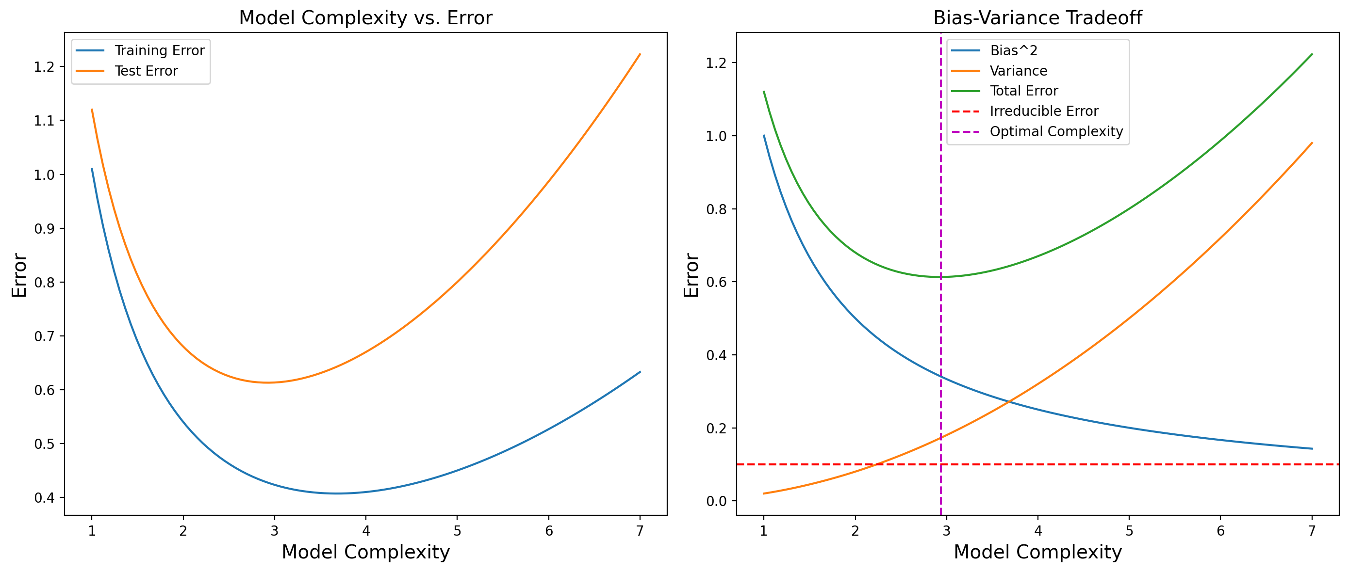
To illustrate the bias-variance tradeoff, we can use a visual representation. Here, we’ll plot the training error and test error as functions of model complexity. Typically, as model complexity increases, the training error decreases, while the test error first decreases and then increases, forming a U-shaped curve.

Graphs include:

1. Model Complexity vs. Error:

   • Plot training error and test error against model complexity.

2. Bias-Variance Decomposition:

   • Plot bias squared, variance, and total error against model complexity.

Interpretation

1. Model Complexity vs. Error:

   • The training error decreases as model complexity increases because the model can better fit the training data.

   • The test error decreases initially but starts to increase after a certain point, indicating overfitting. The test error curve shows a local minimum, reflecting the optimal model complexity where the tradeoff between bias and variance is balanced.

2. Bias-Variance Decomposition:

   • Bias squared decreases with increasing model complexity, as the model becomes more capable of capturing the underlying patterns.

   • Variance increases with model complexity, as the model starts to fit the noise in the training data.

   • The total error curve shows a local minimum at an optimal model complexity, balancing bias and variance. This minimum is marked with a vertical green dashed line.

   • The intersection point of the bias and variance curves is not necessarily the point of minimum total error.

In summary, the optimal model complexity is where the total error is minimized, which takes into account the contributions of bias, variance, and irreducible error. This point is typically where the model has the best balance between underfitting and overfitting.

Mean Squared Error

From many independent imperfect measurements we can easily derive a better one. Here the accent goes on the concept of independence. We say that two events, \(A\) and \(B\), are independent if

\[ \text{P}\left(A\cap B\right) = \text{P}\left(A\right)\cdot\text{P}\left(B\right)\]

Observation: While the above statement is correct, it is also deceivingly simple, and it’s typically hard to use in practice.

Now, assume we have \(n\) independent imperfect, however unbiased, measurements of an object labeled as

\[ x_1, x_2, \dots x_n\]

and we assume that there is an ideal mesurement \(x^*\) and we want to find it. Gauss’ idea is to create an objective function that weighs more heavily larger errors. This can be formalized by assuming that we want to compute a value \(x\) that minimizes the sum of the squared errors/deviances:

\[\text{SSE}\left(x\right)\overset{\Delta}{=} (x-x_1)^2 + (x-x_2)^2 +\dots (x-x_n)^2\]

If we divide by the number of observations, \(n\), we get

\[\text{MSE}\left(x\right)\overset{\Delta}{=} \frac{(x-x_1)^2 + (x-x_2)^2 +\dots (x-x_n)^2}{n}\]

Important: When the number of observations is fixed, \(n\) is just a constant.

So, in this case, we want to determine

\[ \underset{x\,\in\, \mathbb{R}}{\operatorname{argmin}} \text{SSE}(x)\]

that is to say we want the value of \(x\) that yields the minimum of MSE.

To solve the problem, we take the derivative of the MSE with respect to \(x\) and set it equal to zero:

\[ 2(x-x_1) + 2(x-x_2) + \dots 2(x-x_n)=0.\]

When you solve this equation, you get that

\[ x = \frac{x_1+x_2+\dots x_n}{n}\]

This highlights the idea that the average is the best representative of a sample.

The Gradient Descent in 2-D

We want to minimize a cost function that depends on some coefficients. An example in 2-D is

\[L(w_1,w_2): = \frac{1}{n}\sum (y_i - w_1\cdot x_{i1} - w_2\cdot x_{i2})^2\]

Here we have a vector $\(\vec{w}:=(w_1,w_2)\)$

We can think of the vector \(\vec{w}\) having (in this case) two components and a perturbation of \(\vec{w}\) in some direction such as \(\vec{v}.\)

We consider the function \(g(t):=L(\vec{w}+t\cdot \vec{v})\) we get some important ideas:

i. if \(\vec{w}\) is ideal for the cost then \(t=0\) is min of the function \(g\) and so \(g'(0)=0.\)

ii. if \(\vec{w}\) is not minimizing the cost then we want to decrease the function \(g\)

Here we have that $\(g'(t):= \nabla L \cdot \vec{v}\)\( should be negative (because we want to decrease \)g$) and we get a good outcome if

\[\vec{v}:= - \nabla L\]

This means that the coefficients should be updated in the negative direction of the gradient, such as:

\[ w_{new} := \vec{w}_{old} - \text{lr}\cdot\nabla L\]

where “lr” stands for “learning rate.”

The Loss Function (SSE) and its Gradient for n Observations

\[L(w_1,w_2):=\sum_{i=1}^{n}(y_i-w_1\cdot x_{i1} -w_2\cdot x_{i2})^2\]

\[\frac{\partial{L}}{\partial w_1}=\sum_{i=1}^{n} 2\cdot (y_i-w_1\cdot x_{i1} -w_2\cdot x_{i2})\cdot (-x_{i1})\]

### A 2D Example with Partial Derivatives and One Observation

If

\[L(w_1,w_2) = (y-w_1\cdot x_1-w_2\cdot x_2)^2\]

What are the partial derivatives of \(L\) with respect to \(w_1\) and \(w_2\)?

\[\frac{\partial{L}}{\partial{w_1}}= 2\cdot(y-w_1\cdot x_1-w_2\cdot x_2)\cdot (-x_1)\]

\[\frac{\partial{L}}{\partial{w_2}}= 2\cdot(y-w_1\cdot x_1-w_2\cdot x_2)\cdot (-x_2)\]

Code Applications

---

import os
if 'google.colab' in str(get_ipython()):
  print('Running on CoLab')
  from google.colab import drive
  drive.mount('/content/drive')
  os.chdir('/content/drive/My Drive/Data Sets')
  !pip install -q pygam
else:
  print('Running locally')
  os.chdir('../Data')

Running on CoLab
Mounted at /content/drive
     ━━━━━━━━━━━━━━━━━━━━━━━━━━━━━━━━━━━━━━━━ 522.0/522.0 kB 7.6 MB/s eta 0:00:00
?25h

# Setup Libraries
import numpy as np
import matplotlib.pyplot as plt
import matplotlib as mpl
%matplotlib inline
%config InlineBackend.figure_format = 'retina'
import matplotlib.pyplot as plt

Example with Functions and Classes

Let’s create some examples in Python:

Example 1 Create a function whose graph intersects the line \(y=0.5\) exactly three times.

Solution: We think of a simple possible design that accomodates the requirement such as the construct of a third degree polynomial:

\[ p(x) = (x-1)\cdot(x-2)\cdot(x-3)+0.5 \]

def myfunction(x):
  return (x-1)*(x-2)*(x-3)+0.5

myfunction(2.7)

0.14300000000000007

myfunction(t)

Example 2 Create a piecewise defined function with three different cases.

Solution: Again, we can think of a simple example such as

\[\begin{split} f(x) = \begin{cases} x &\text{if}\,\,\,0<x<1\\ \sqrt{x} & \text{if}\,\,\,1\leq x<2\\ \sin(x) & \text{if}\,\,\,2\leq x \,\,\text{or}\,\, x\leq0 \end{cases} \end{split}\]

Hint: for Python programming consider if, elif and else statements.

def f(x):
  if 0<x<1:
    return x
  elif 1<=x<2:
    return np.sqrt(x)
  else:
    return np.sin(x)

g =np.vectorize(f)

g([3.4,1.2,2.6,0.3])

array([-0.2555411 ,  1.09544512,  0.51550137,  0.3       ])

Example 3 A simple class.

# a very simple example
class Honda:
  mileage = 37
  color = 'red'
  year = 2019
  model = 'Civic'
  def __init__(self,color,year,model,mileage):
    self.year = year
    self.model = model
    self.mileage = mileage
    self.color = color

Example 4 A Fibonacci sequence.

Iterative approach to generating the Fibonacci sequence, i.e. the sequence \((f_n)\) of integers such that $\(f_0=0,\,\, f_1=1\,\,\, \text{and}\,\, f_{n+1}=f_n+f_{n-1}\)\( for all \)n\geq 1.$

class Fib:
  def __init__(self,a=0,b=1):
    self.a = a
    self.b = b
  def update(self):
    self.a, self.b = self.b, self.a + self.b
    self.current = self.b

myfib=Fib(a=-1,b=2)

myfib.update()
myfib.current

1

class FibNumbers:
  def __iter__(self):
    self.a = 0
    self.b = 1
    return self

  def __next__(self):
    self.a, self.b = self.b, self.a + self.b
    return self.b

myclass = FibNumbers()

iter(myclass)

<__main__.FibNumbers at 0x7a1ead26e410>

next(myclass)

21

An Example of Gradient Descent with Contour Plots

# here we generate many equally spaced points
x1 = np.linspace(-10.0, 10.0, 201)
x2 = np.linspace(-10.0, 10.0, 201)
# here we make an objective function
X1, X2 = np.meshgrid(x1, x2)
Y = np.sqrt(X1**2/9 + X2**2/4)

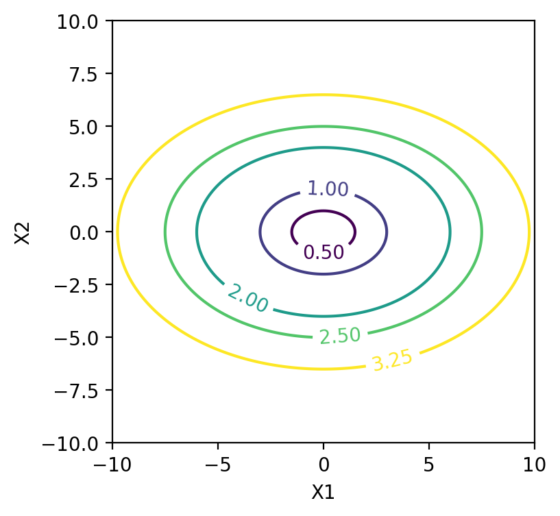
Here we have the function:

\[F(x_1,x_2):=\sqrt{\frac{x_1^2}{9}+\frac{x_2^2}{4}}\]

What shape is implied by the equation

\[\frac{x_1^2}{9}+\frac{x_2^2}{4}=k\]

Here the function is $\(f(x_1,x_2):=\frac{(x_1)^2}{9}+\frac{(x_2)^2}{4}\)$

The level curve is the geometric locus of points \((x_1,x_2)\) such that

\[f(x_1,x_2)=l\]

The gradient of \(f\) is labeled by \(\nabla(f)\) and is the vector of partial derivatives with respect to \(x1\) and \(x2\)

\[\nabla(f):=\left(\frac{\partial{f}}{\partial{x1}},\frac{\partial{f}}{\partial{x2}}\right)=\left(\frac{2x1}{9},\frac{x2}{2}\right)\]

fig = plt.figure(figsize=(4,4))
ax = plt.gca() #you first need to get the axis handle
ax.set_aspect(1)
cm = mpl.colormaps['coolwarm']
plt.scatter(X1, X2, c=Y, cmap=cm)
plt.show()

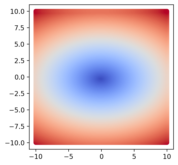
fig = plt.figure(figsize=(4, 4))
ax = plt.gca() #you first need to get the axis handle
ax.set_aspect(1)
levels = [0.5,1,2,2.5,3.25]
cp = plt.contour(X1, X2, Y,levels) # here we show some of the level curves
plt.clabel(cp, inline=1, fontsize=10)
plt.xlabel('X1')
plt.ylabel('X2')
plt.show()

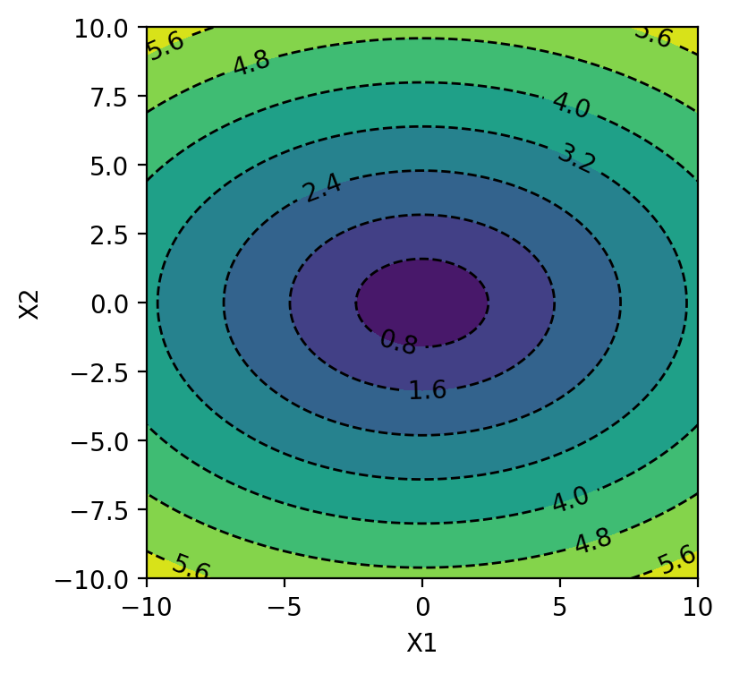
plt.figure(figsize=(4,4))
ax = plt.gca() #you first need to get the axis handle
ax.set_aspect(1)
cp = plt.contour(X1, X2, Y, colors='black', linestyles='dashed', linewidths=1)
plt.clabel(cp, inline=1, fontsize=10)
cp = plt.contourf(X1, X2, Y, )
plt.xlabel('X1')
plt.ylabel('X2')
plt.show()

Code for Plotting the Bias - Variance Tradeoff

# Generate example data
model_complexity = np.linspace(1, 7, 100)
bias_squared = 1 / model_complexity
variance = model_complexity**2 / 50
irreducible_error = np.full_like(model_complexity, 0.1)
total_error = bias_squared + variance + irreducible_error

# Find the index of the minimum total error
min_total_error_index = np.argmin(total_error)

# Plotting Model Complexity vs. Error
plt.figure(figsize=(14, 6))

# Subplot 1: Training and Test Error vs. Model Complexity
plt.subplot(1, 2, 1)
train_error = bias_squared + variance / 2  # Hypothetical training error
test_error = total_error  # Hypothetical test error

plt.plot(model_complexity, train_error, label='Training Error')
plt.plot(model_complexity, test_error, label='Test Error')
plt.xlabel('Model Complexity',fontsize=14)
plt.ylabel('Error',fontsize=14)
plt.title('Model Complexity vs. Error',fontsize=14)
plt.legend()

# Subplot 2: Bias-Variance Decomposition
plt.subplot(1, 2, 2)
plt.plot(model_complexity, bias_squared, label='Bias^2')
plt.plot(model_complexity, variance, label='Variance')
plt.plot(model_complexity, total_error, label='Total Error')
plt.axhline(y=0.1, color='r', linestyle='--', label='Irreducible Error')
plt.axvline(x=model_complexity[min_total_error_index], color='m', linestyle='--', label='Optimal Complexity')
plt.xlabel('Model Complexity',fontsize=14)
plt.ylabel('Error',fontsize=14)
plt.title('Bias-Variance Tradeoff',fontsize=14)
plt.legend()

plt.tight_layout()
plt.savefig('bias_variance_tradeoff.png',dpi=300,bbox_inches='tight')
plt.show()