Nonparamatric Methods #

The Nadaraya-Watson Regressor #

Main Idea: Estimate a conditional mean (expected value) given the input variables.

\[\large{ \mathbb{E}[Y| X=x]=\sum\limits_{i=1}^nW_{i}(x)y_i} \]

If we have estimates for the joint probability density $f$ and the marginal density $f_X$ we consider:

\[\large{ m(x)=\mathbb{E}[y| X=x]=\int y f_{Y| X=x}(y)\,\mathrm{d}y=\frac{\int yf(x,y)\,\mathrm{d}y}{f_X(x)}\tag{1} } \]

where $X$ is the input data (features) and $Y$ is the dependent variable.

We approximate the joint probability density function by using a kernel:

\[\large{ \begin{align} \hat{f}(x,y;\mathbf{h})=\frac{1}{n}\sum_{i=1}^n K_{h_1}(x-x_{i})K_{h_2}(y-y_{i}). \end{align}} \]

The marginal density is also approximated in a similar way:

\[\large{ \hat{f}_X(x;h_1)=\frac{1}{n}\sum_{i=1}^nK_{h_1}(x-x_{i})}. \]

By substituting these approximations into equation (1) we obtain:

\[\begin{split}{ \begin{align*} \frac{\int y \hat{f}(x,y;\mathbf{h})\,\mathrm{d}y}{\hat{f}_X(x;h_1)}=&\,\frac{\int y \frac{1}{n}\sum_{i=1}^nK_{h_1}(x-X_i)K_{h_2}(y-y_i)\,\mathrm{d}y}{\frac{1}{n}\sum_{i=1}^nK_{h_1}(x-x_i)}\\ =&\,\frac{\frac{1}{n}\sum_{i=1}^nK_{h_1}(x-x_i)\int y K_{h_2}(y-y_i)\,\mathrm{d}y}{\frac{1}{n}\sum_{i=1}^nK_{h_1}(x-x_i)}\\ =&\,\frac{\frac{1}{n}\sum_{i=1}^nK_{h_1}(x-x_i)y_i}{\frac{1}{n}\sum_{i=1}^nK_{h_1}(x-x_i)}\\ =&\,\sum_{i=1}^n\frac{K_{h_1}(x-x_i)}{\sum_{i=1}^nK_{h_1}(x-x_i)}y_i. \end{align*}} \end{split}\]

Thus the conditional mean $\mathbb{E}[Y| X=x]$ can be seen as a weighted average of $y_i$:

\[\large{ \mathbb{E}[Y| X=x]=\sum\limits_{i=1}^nW_{i}(x)y_i} \]

where

\[\large{ \begin{align*} W_{i}(x):=\frac{K_h(x-x_i)}{\sum_{i=1}^nK_h(x-x_i)}. \end{align*}} \]

This is to say that the Nadaraya-Watson estimator is a local mean of $Y$ around $X=x_i.$

Functional Data Analysis - GAMs #

The main idea of generalized additive models (GAMs) is based on the assumption that

\[\large \mathbb{E}\left[Y|X=x_i\right]=\beta_0+f_1(x_{i1})+f_2(x_{i2})+...+f_p(x_{ip})\]

By comparison, a linear model is

\[\large \mathbb{E}\left[Y|X=x_i\right]=\beta_0+\beta_1\cdot x_{i1}+\beta_2\cdot x_{i2}+...+\beta_p\cdot x_{ip}\]

We consider a regularized maximum likelihood approach for the generalized additive model

\[\large y_i = c +\sum\limits_{j=1}^{p}f_j(x_i^{(j)}) + \epsilon_i \]

and for standardization we assume

\[\large \sum\limits_{i=1}^{n}f_j(x_i^{(j)})=0 \]

For classificaiton problems we can use:

\[\large g\left(\mathbb{P}\left[Y=c|X=x_i\right]\right) = c +\sum\limits_{j=1}^{p}f_j(x_i^{(j)}) \]

where $g$ is a link function, e.g. the inverse of the logistic sigmoid.

To prevent overfitting, we consider a sparsity-smoothness regularization:

\[\large J(f_i) = \lambda_1\sqrt{\|f_j\|^2_n+\lambda_2I^2(f_j)} \]

where the following term is designed to control the rapid accelerations/decelerations.

\[\large I^2(f_j)=\int(f''_j(x))^2dx \,\,\, \text{and}\,\,\,\|f\|^2_n=\frac{1}{n}\sum\limits_{i=1}^{n}f_i^2. \]

The objective function is

\[\large \left \|y-\sum\limits_{j=1}^{p}f_j\right\|_n^2 + \sum\limits_{j=1}^{p}J(f_j). \]

and this is to minimize over a suitable class of functions $\mathcal{F}.$

Cubic Splines#

What we need:

we need the tools, the building blocks for constructing any nonlinearity we want.
we need a good validation mechanism.
we need an efficient implementation of such tools in programming languages, e.g. Python.

The main idea is to use third degree polynomial functions, such as

\[ s_i(x)=a_i(x-x_i)^3+b_i(x-x_i)^2+c_i(x-x_i)+d_i \]

for $i=1,2,...,n-1$ and $x_i$ are data points of the same feature. It is quite obvious that we have:

\[ s'_i(x) = 3a_i(x-x_i)^2+2b_i(x-x_i)+c_i \]

and $$ s''_i(x)=6a_i(x-x_i)+2b_i $$

So we create

\[\begin{split} S(x)= \begin{cases} s_1(x) &\text{if}& x_1\leq x < x_2 \\ s_2(x) &\text{if}& x_2\leq x < x_3 \\ ...\\ s_n(x) &\text{if}& x_{n-1}\leq x < x_n \end{cases} \end{split}\]

We generally want the following properties to hold:

$S(x)$ is continuous on $[x_1,x_n].$
$S'(x)$ is continuous on $[x_1,x_n].$
$S''(x)$ is continuous on $[x_1,x_n].$

And of course, we want to interpolate some data points:

\[ S(x_i)=y_i \]

and that is to say that

\[ y_i= d_i. \]

In order to make the curve smooth across the interval, the derivatives must be equal at the stitching points:

\[ s'_i(x_i) = s'_{i-1}(x_i). \]

Let $M_i:=2b_i$ and $h=x_{i+1}-x_i$. After some sensible calculations we get the following matrix equation:

\begin{align} \begin{bmatrix} 1 & 4 & 1 & 0 & \dots & 0 & 0 & 0 & 0\ 0 & 1 & 4 & 1 & \dots & 0 & 0 & 0 & 0\ 0 & 0 & 1 & 4 & \dots & 0 & 0 & 0 & 0\ \vdots & \vdots & \vdots & \vdots & \ddots & \vdots & \vdots & \vdots & \vdots\ 0 & 0 & 0 & 0 & \dots & 4 & 1 & 0 & 0\ 0 & 0 & 0 & 0 & \dots & 1 & 1 & 1 & 0\ 0 & 0 & 0 & 0 & \dots & 0 & 1 & 4 & 1 \end{bmatrix} \begin{bmatrix} M_1\ M_2\ M_3\ M_4\ \vdots\ M_{n-3}\ M_{n-2}\ M_{n-1}\ M_n \end{bmatrix} =\frac{6}{h^2} \begin{bmatrix} y_1-2y_2+y_3\ y_2-2y_3+y_4\ y_3-2y_4+y_5\ \vdots\ y_{n-4}-2y_{n-3}+y_{n-2}\ y_{n-3}-2y_{n-2}+y_{n-1}\ y_{n-2}-2y_{n-1}+y_{n} \end{bmatrix} \end{align}

which linear system has $n-2$ rows and $n$ columns, so it is underdetermined. We can solve this system by imposing some extra conditions.

One easy condition is $M_1=M_n=0$ and what we get is referred to as Natural Splines.

Generalized Additive Modeling#

The assumption is that

\[ y_i = \sum\limits_{j=1}^{p}S_j(x_{ij}) +\text{noise} \]

and of course, ideally, the mean of the noise should be 0; here $p$ is the number of features.

So we get

\[\mathbb{E}\left[Y| X=x_i \right]= \sum\limits_{j=1}^{p}S_j\left(x_{ij}\right)\]

In this way we can reduce the nonlinear problem to a multiple linear one, however the tradeoff is that we have many more weigths to determine !

This is the reson we need very good methods of regularization and variable selection.

Model Complexity#

Let’s assume that we have N knots. For each feature we fit N cubic splines. This means that we subdivide the range of each feature into N eaqually spaced intervals. On each such interval you have a cubic polynomial. For the same feature the cubic polynomials connect smoothly at the knots.

Model Complexity: we determine 4 coefficients for each cubic. We have N knots for each feature so in the end we have 4Np coefficients (weights) to determine.

Number of Splines If the data has $n$ observations, we may consider

\[\left\lceil \log_2(n)\right\rceil\]

Code Applications#

Setup#

import os
if 'google.colab' in str(get_ipython()):
  print('Running on CoLab')
  from google.colab import drive
  drive.mount('/content/drive')
  os.chdir('/content/drive/My Drive/Data Sets')
  !pip install -q pygam
else:
  print('Running locally')
  os.chdir('../Data')

Running on CoLab
Drive already mounted at /content/drive; to attempt to forcibly remount, call drive.mount("/content/drive", force_remount=True).

# library imports
import numpy as np
import pandas as pd
from math import ceil
from scipy import linalg
from sklearn.linear_model import LinearRegression, Ridge, Lasso, ElasticNet
from sklearn.metrics import mean_absolute_error, mean_squared_error as mse, r2_score
from sklearn.preprocessing import StandardScaler, MinMaxScaler
from sklearn.model_selection import GridSearchCV,train_test_split as tts, KFold

from pygam import LinearGAM

from sklearn.pipeline import Pipeline

%matplotlib inline
%config InlineBackend.figure_format = 'retina'
import matplotlib.pyplot as plt
from scipy.optimize import minimize
from matplotlib import pyplot

from nadaraya_watson import NadarayaWatson, NadarayaWatsonCV

Synthetic Data Applications#

rng = np.random.RandomState(123)

# #############################################################################
# Generate sample data
X = 5 * rng.rand(120, 1)
y = 2*np.sin(3*X).ravel()

# Add noise to targets
#y[::4] += 3 * (0.5 - rng.rand(X.shape[0] // 6))

y = y + 0.5*np.random.normal(0,1,len(X))

X_plot = np.linspace(0, 5, 1000)[:, None]

# Fit regression model
train_size = 100
param_grid=[dict(kernel=['polynomial'], degree=np.arange(1, 3)),dict(kernel=['rbf'], gamma=np.logspace(-4, 1, 100))]

# use the sklearn gridsearch
nw_gs = GridSearchCV(NadarayaWatson(), cv=10, param_grid=param_grid)

# use the internal LOO (leave-one-out cross-validation)
nw_cv = NadarayaWatsonCV(param_grid)

# fit k-fold using GridSearch
nw_gs.fit(X[:train_size], y[:train_size])


print("\toptimal bandwidth found: %.2f" % nw_gs.best_estimator_.gamma)

# fit leave-one-out using NadarayaWatsonCV

nw_cv.fit(X[:train_size], y[:train_size])

print("\toptimal bandwidth found: %.3f" % nw_cv.gamma)

# predict
y_gs = nw_gs.predict(X_plot)
y_cv = nw_cv.predict(X_plot)

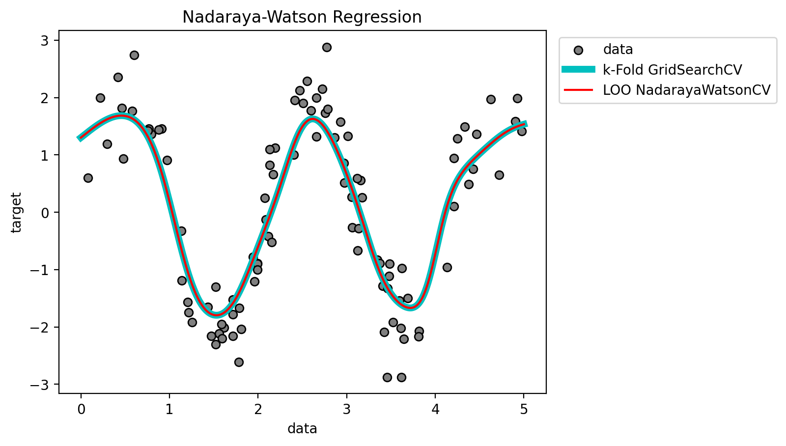
plt.scatter(X[:100], y[:100], c='grey', label='data', zorder=1,
            edgecolors=(0, 0, 0))
plt.plot(X_plot, y_gs, 'c', lw=5, label='k-Fold GridSearchCV')
plt.plot(X_plot, y_cv, 'r', lw=1.5, label='LOO NadarayaWatsonCV')
plt.xlabel('data')
plt.ylabel('target')
plt.title('Nadaraya-Watson Regression')
plt.legend(loc = 9, bbox_to_anchor=(1.25,1))
#plt.savefig('fig3.png',bbox_inches='tight',dpi=300)
plt.show()

	optimal bandwidth found: 10.00
	optimal bandwidth found: 10.000

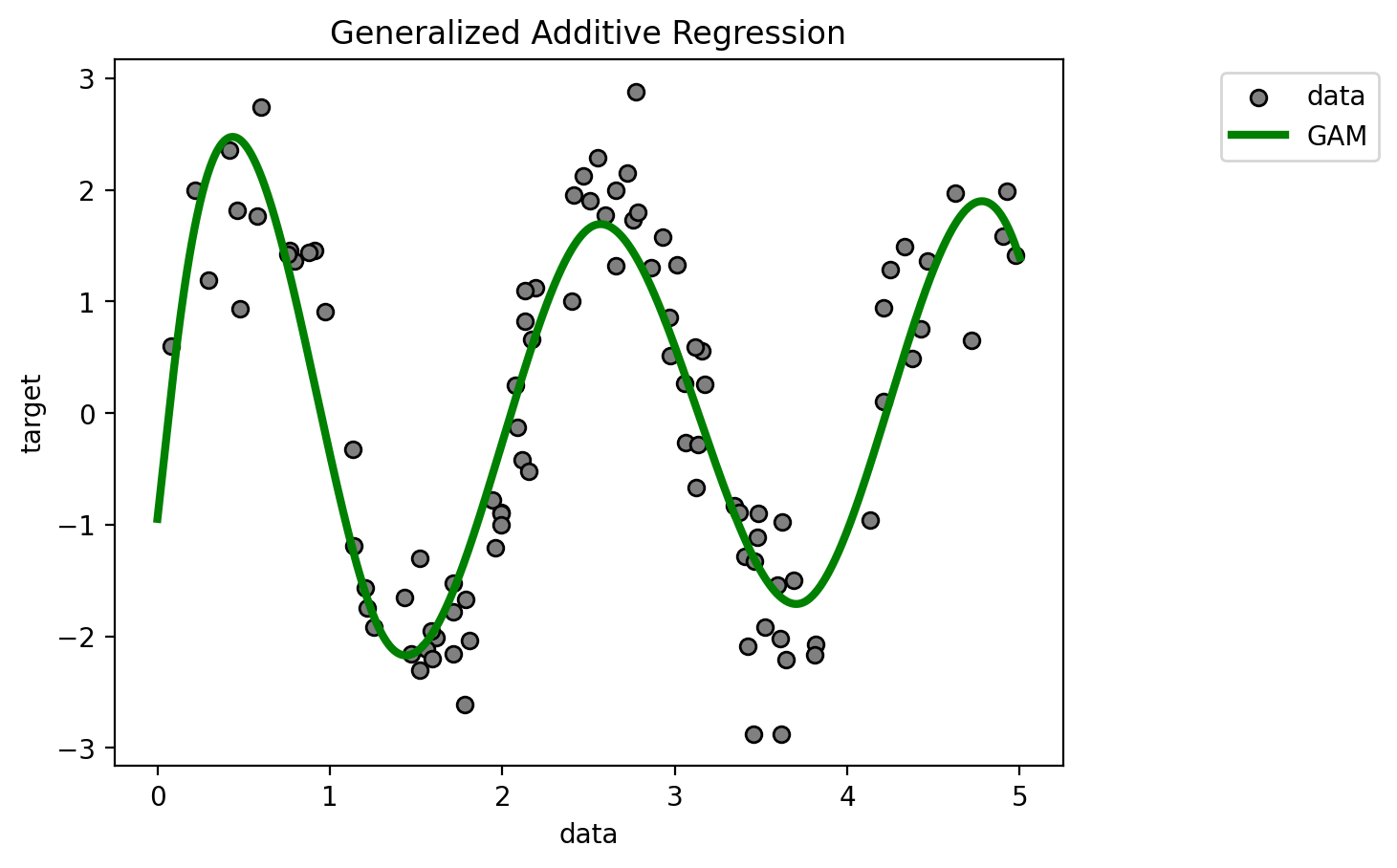
_images/Nonparametric_Methods_GAMs__old_9_1.png

# here you have to guess the "right" number of splines: since we have about 100 data points we should test 6 or 7 splines
gam = LinearGAM(n_splines=ceil(np.log2(len(X[:train_size])))).gridsearch(X[:train_size], y[:train_size],objective='GCV')

100% (11 of 11) |########################| Elapsed Time: 0:00:00 Time:  0:00:00

y_gams = gam.predict(X_plot)
plt.scatter(X[:100], y[:100], c='grey', label='data', zorder=1,
            edgecolors=(0, 0, 0))
plt.plot(X_plot, y_gams, 'g', lw=3, label='GAM')
plt.xlabel('data')
plt.ylabel('target')
plt.title('Generalized Additive Regression')
plt.legend(loc = 9, bbox_to_anchor=(1.25,1))
plt.show()

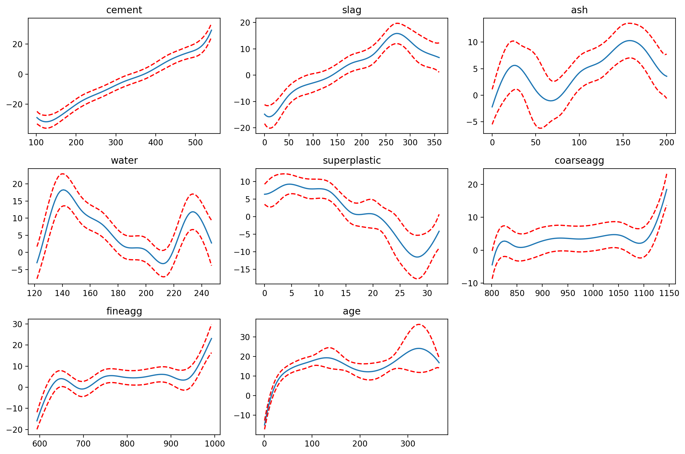
_images/Nonparametric_Methods_GAMs__old_11_0.png

Applications with Real Data#

data_concrete = pd.read_csv('concrete.csv')

x = data_concrete[data_concrete.columns[:-1]]
y = data_concrete[data_concrete.columns[-1]]

ceil(np.log2(len(x)))

# compute the number of knots
n_knots = ceil(np.log2(len(x)))

gam = LinearGAM(n_splines=n_knots).gridsearch(x.values, y.values,objective='GCV')

100% (11 of 11) |########################| Elapsed Time: 0:00:04 Time:  0:00:04

fig = plt.figure(figsize=(8,12))
titles = x.columns

fig.set_figheight(8)
fig.set_figwidth(12)

for i, term in enumerate(gam.terms):
    if term.isintercept:
        continue
    XX = gam.generate_X_grid(term=i)
    pdep, confi = gam.partial_dependence(term=i, X=XX, width=0.95)
    ax = fig.add_subplot(3, 3, i+1)
    ax.plot(XX[:, term.feature], pdep)
    ax.plot(XX[:, term.feature], confi, c='r', ls='--')
    ax.set_title(titles[i])
    fig.tight_layout()
plt.show()

_images/Nonparametric_Methods_GAMs__old_18_0.png

gam.terms

s(0) + s(1) + s(2) + s(3) + s(4) + s(5) + s(6) + s(7) + intercept

AI for Fusion Energy Summer School (2024)

Nonparamatric Methods

Contents